The problem is a so-called shortest path computation on a graph. Various kinds of shortest path computations have applications ranging from automatic driving directions to playing "six degrees of Kevin Bacon." Here, you'll solve a particular version called "all-pairs shortest paths," which takes a directed graph with lengths on the edges and tells you the shortest distance from every vertex to every other vertex.
You are given a graph with vertices and edges. Each edge is labelled with a number called its "length," which you can think of as the cost (in time or distance or dollars) of going from the vertex at the tail of the edge to the vertex at the head of the edge. Lengths are real numbers, and they have to be positive or zero. The edges are directed--that is, if there is an edge from vertex a to vertex b, there may or may not be an edge from b to a, and even if both edges are there, they can have different lengths. Formally speaking, the input is an "edge-weighted directed graph" with non-negative weights.
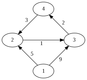
One way to specify such a graph is to draw a picture with circles for the vertices and arrows for the edges. The figure here shows a graph with four vertices and five edges.
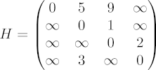
Another way to specify an edge-weighted graph is to write down a two-dimensional table, or matrix H, in which H(i,j) is the length of the edge from vertex i to vertex j. The figure shows the matrix H for the given graph. Notice that the diagonal entries H(i,i) are all zero (meaning that there's no cost if you don't move from the vertex you're at), and that H(i,j) is infinity if there is no edge from vertex i to vertex j.
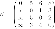
The problem is to compute, for every pair (i,j) of vertices, the cost of the shortest path (meaning the cheapest, not the fewest steps) of directed edges that leads from i to j. The figure shows the shortest path costs as the matrix S. Notice that S(i,j) can be smaller than H(i,j) -- for example, it costs H(1,3) = 9 to go from vertex 1 to vertex 3 directly, but it costs only S(1,3) = 6 to go from 1 to 2 to 3. Also notice that there are some cases where you can't get there from here -- for example, S(2,1) is still infinity, because there is no path of edges from vertex 2 to vertex 1.
There are several different algorithms to solve the all-pairs shortest path problem; maybe the best-known is the Floyd-Warshall algorithm (you can find it in Wikipedia). However, the best algorithm for parallel implementation, at least on a GPU, is a less well-known one called the recursive Kleene, or R-Kleene, algorithm. There is a Matlab implementation "apsp.m" of R-Kleene on the course web site here. Try typing the 4-by-4 matrix H above into Matlab and saying "apsp(H)".
The key idea of R-Kleene is that there is a connection between multiplying matrices and concatenating paths in a graph. Suppose X is an n1-by-n2 matrix whose rows represent a set R of n1 vertices and whose columns represent a set S of n2 vertices, and X(i,k) is the cost of going from vertex i in R to vertex k in S. (Here R and S can be the same set of vertices, or different sets.) Suppose Y is an n2-by-n3 matrix whose entries Y(k,j) give the cost of going from a vertex k in S to a vertex j in yet another set T, with n3 vertices. (Again T could be the same as R and S, or not.) Then the minimum cost Z(i,j) of going from a vertex i in R to a vertex j in T by way of a vertex in S is given by the following expression, which takes the minimum over all possible intermediate vertices:
Z(i,j) = min( X(i,1)+Y(1,j), X(i,2)+Y(2,j), X(i,3)+Y(3,j), ..., X(i,n2)+Y(n2,j) ).
This expression looks an awful lot like the expression for multiplying two matrices X and Y to get matrix Z. Indeed, if we changed "+" to "*" and we changed "min" to "sum", we would have Z = X*Y. So, we can write code to compute Z from X and Y that looks exactly like matrix-multiplication code except for using (min,+) in place of (+,*) in the innermost loop. The sample Matlab code "min_plus.m" on the course web site does exactly that.
R-Kleene uses this (min,+) matrix multiplication several times, as you'll see in the code "apsp.m". It works recursively, by breaking the matrix H up into four blocks, H = [A B ; C D]. Block A has costs of edges between vertices in the first half of the graph; block D has costs of edges between vertices in the second half. Block B has costs of edges from the first half to the second half, and block C has costs of edges back from the second half to the first half. R-Kleene first calls itself recursively on A, to get shortest paths that never leave the first half of the graph; then it updates B, C, and D to account for paths that go through A; then it makes another recursive call on D, to find shortest paths from one vertex in D to another (which now includes paths that go through A on the way); then it updates B and C and finally A to account for those paths too. You might want to make up some graphs and experiment with the Matlab code to get an idea of what it's doing. You can also find a few slides with diagrams here.
For the parallel version of this algorithm, you will essentially parallelize the (min,+) "matrix multiplication" routine, since that's where all the action is. How you do this is up to you, but here are a few hints:
You should write a sequential C code as well as a CUDA code for this problem. Try both of them on very small graphs (like H in the example above) to convince yourself that they're correct.
Then, benchmark the CUDA code on a sequence of larger and larger problems (up to the largest you can fit in GPU memory). Analyze (with both tables and graphs) the scaling of the parallel code, and also how it compares to the sequential code. What are your conclusions? In your report, describe the process you went through and what you learned about tuning CUDA for performance.