CS190N Numb3rs -- The Pilot

The situation:

Our math-hero Charlie draws the analogy between the locations of his strikes and the locations of water droplets from a sprinkler. Discussion Question: What assumptions are being made when we draw this analogy? Given the locations of all the droplets, we would have a very good idea where the sprinkler is located!

Now, how can we re-express this type of problem into something more mathematical, a setting in which we can use, well, numb3rs? I think you'll agree that a natural starting point would be to plot the strikes as a set of points in the xy-plane. We're looking for the "source" of the points, something like the "center." Is there a good way to measure the center of a set of points? Assuming that the points really are "randomly" distributed in some sense about the center, how closely will the center that we measure approximate the true center? Good questions!

Walk the line

How does this work? It relates to the so-called normal distribution, which is a way of describing how numbers are distributed. You are probably already familiar with the uniform distribution on [0,1], whether you know it or not: It is the distribution that functions like rand() in C are supposed to use. The uniform distribution has the property that numbers near the center and away from the center all have an equal chance of being picked. Graphically, this distribution looks like a horizontal line of height 1, above the interval x=0 to x=1. (Note: This picture is really describing what histograms of samples from this population would look like if you had "perfectly representative" samples of large size, scaled so that the total area is equal to 1.)

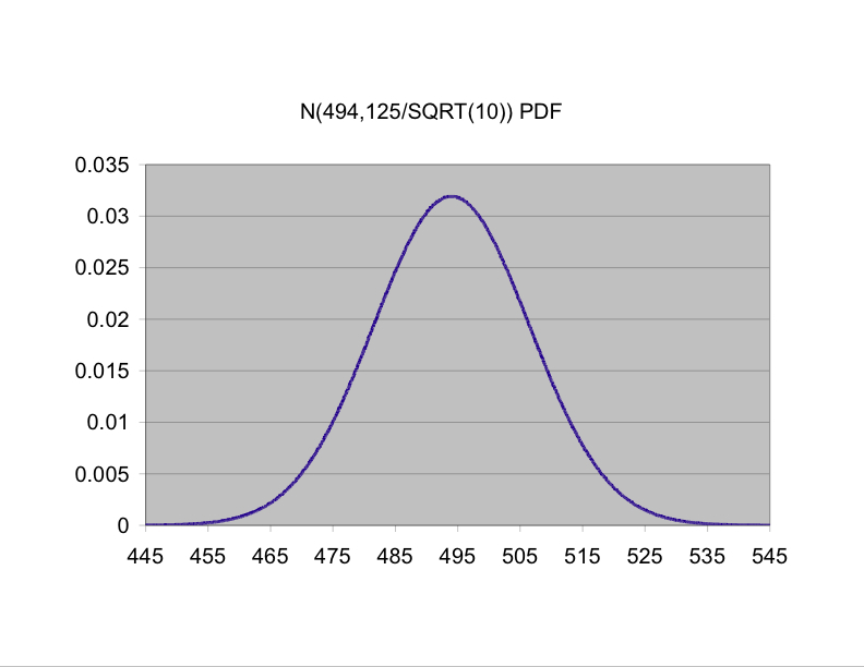
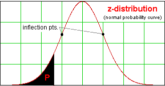
In the real world, a lot of things are not distributed uniformly. Going back to the example of heights of male UCSB students, we would be much more likely to see values near, say 5'10" than near 7'1". The way the heights are distributed would be roughly symmetric, tall near the middle, and tapering off at the ends in the famous "bell-shaped" pattern: in other words, normally distributed populations have more measurements near the center and fewer far from the center. Normal distributions can be centered anywhere; the mean or population average, which we call &mu for short, of a normal distribution is located right at the peak of the bell. Also, the "bell" can be tall and thin or shorter and wider; the "spread" of a normal distribution is measured by its standard deviation, &sigma, which is the distance from the mean to either inflection point on the "bell."

On the right-had side of this page is a cute applet to graph a normal distribution having any mean and standard deviation (which they call A and B for some bizarre reason!!) that you choose. They also have a mathematical expression (labeled "PDF") defining the equation for a normal distribution with given &mu = A and &sigma = B, but we won't worry a huge amount about that at the moment. A couple of things we do need to know about the normal distribution are that

• You can turn any normal distribution into any other via a shift and a scaling factor.
• For any normal distribution, 95% of the values lie within about 1.96 standard deviations of the mean. We can use a normal table, like this one here, in order to figure out how much of the population lies within whatever part of the curve you're interested in. The negative values along the left-hand column indicate that many standard deviations below the mean. Since the curve is symmetric, you can figure out the value of P for values above the mean quite easily. For example, to figure out what part of the population is less than 1.5 standard deviations above the mean, look for −1.5, and find the value .06681. This tells us how much of the population has a value that is smaller than a value of 1.5 standard deviations below the mean, so by symmetry, .06681 of the population is greater than 1.5 standard deviations above the mean. Thus, the remaining .93319, or about 93.3%, of the population has a value less than 1.5 standard deviations above the mean. (Helpful hint: If you take a few minutes with this table and understand how the .0250 in the −1.96 entry relates to the 95% mentioned at the beginning of this item, those will be minutes well spent -- and I'm not just talking Scooby-Doo well spent, I'm talking Gilligan's-Island well spent! To test your insight, answer this one for me: How many standard deviations on either side of the mean do you have to go in order to encompass 90% of the population? Answer: About 1.645.)
• In light of the above two bullet points, a common trick for a measurement from a population that is normally distributed data is to subtract the mean and divide by the standard deviation. What this does, essentially, is to convert the population to a "standard normal" distribution with mean 0 and standard deviation 1; the number to which our measurement gets transformed is called its z-score, and the z-score of the measurement is the thing you look up in the above table. In other words, a measurement's z-score tells you how many standard deviations it is above or below the mean. We could do everything with z-scores, but I think that just approaching things directly forces you to think clearly about what you're doing, and also leads to fewer careless mistakes.

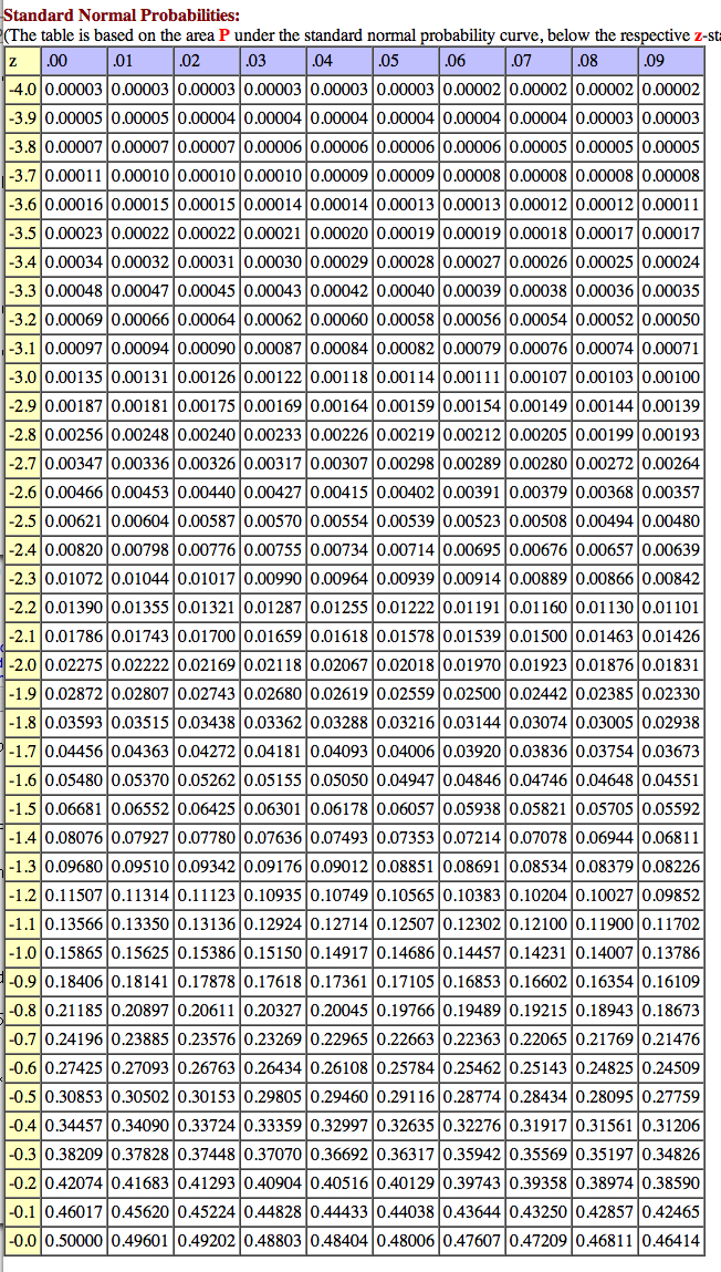
For now, let's go back to our problem about the heights of male students. Suppose that someone has told you that their heights are normally distributed with standard deviation 2 inches. Then, as noted above, 95% of the population will be within 1.96 &sdot 2 = 3.92 inches of the mean, whatever the mean is. Formally, we would say that if you choose a male student at random, the probability that his height is within 3.92 inches of the mean is 95%, or .95. But the really useful observation is that the tail also wags the dog: If the randomly chosen student's height is within 3.92 inches of the mean, then the mean is within 3.92 inches of that student's height! I know that last sentence looks obvious, but chew on it for a minute. Go ahead. I'll wait for you. OK, so even if you know nothing about the mean, you can get information about it by choosing a male student at random and measuring his height: You are 95% confident that the average is somewhere within 3.92 inches of that student's height. Suppose that your randomly chosen student is 5'9"; you are then 95% confident that the average height of all male students is between about 5'5" and about 6'1". It will be useful to keep in mind the difference between probability and confidence. Probability is about what's going to happen with a random event, while confidence is about a non-random thing, in this case the average height of all students, that is unknown.

Sample Means have Distributions, Too

How do we gain more certainty about the mean height? Why, we collect more data, of course -- we increase our sample size. If you think about it for a minute, I think you'll agree that it makes sense that the bigger the sample, the closer its average is likely to be to the average of the whole population - for example, it's perfectly possible to choose a student randomly who is 6'6", but it's practically impossible to choose 100 students at random and have their average height be 6'6"! The question is "How much more certainty do we gain?" Let's denote the mean of a sample by x, as opposed to the mean &mu of the whole population. Now, let's imagine the process of taking a bunch of random samples with a specific number of students, say n, in each sample, and measuring their means. These are random numbers, just as the heights of randomly chosen male students are, but what are the characteristics of these sample means? More fun facts:

• The sample means will still have the same mean &mu as the population (no surprise there, right??), and the standard deviation of the sample means will be &sigma⁄&radicn -- it gets smaller as the sample we consider gets larger! Getting back to our favorite(!!) example, if you have a random sample of 100 UCSB males and find their mean height, the standard deviation of that process has gone down to 2⁄&radic100 = 0.2, so now you're 95% confident that the actual mean height is within 1.96 &sdot 0.2, or about 0.4, inches of the mean of your sample.
• This one is kind of a miracle: Even if your original population didn't have a normal distribution, the distribution of the sample mean becomes more and more normal for larger and larger samples. Let's take a look at this in action for our old pal the uniform distribution on [0,1]. I used this code to take 1000 samples of 2 numbers from this distribution and recorded the sample means in this file. To run the code, compile it using the makefile and then execute

  ./uniform_sample -n 2 -k 1000
  

  which says to make 1000 samples of size 2 and to take the sample mean from each. Then I made a histogram using a histogramming program and gnuplot, but you can use this nifty web page. It looked like this:

  

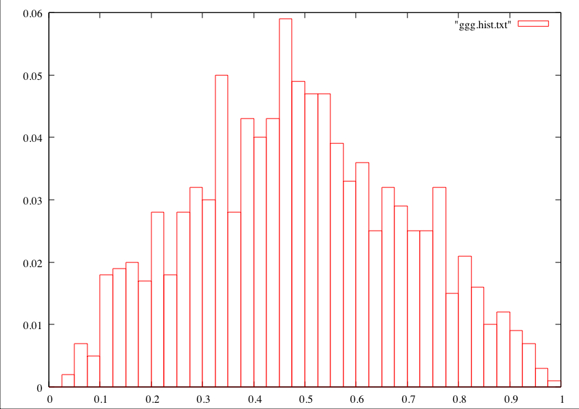
  I think you'll agree that this is peaked in the middle, yet it doesn't really have a "bell shape" like the above picture of an ideal normal distribution. Now, if I do it with 1000 samples of size 20, here's what a histogram of the sample means looks like.

  

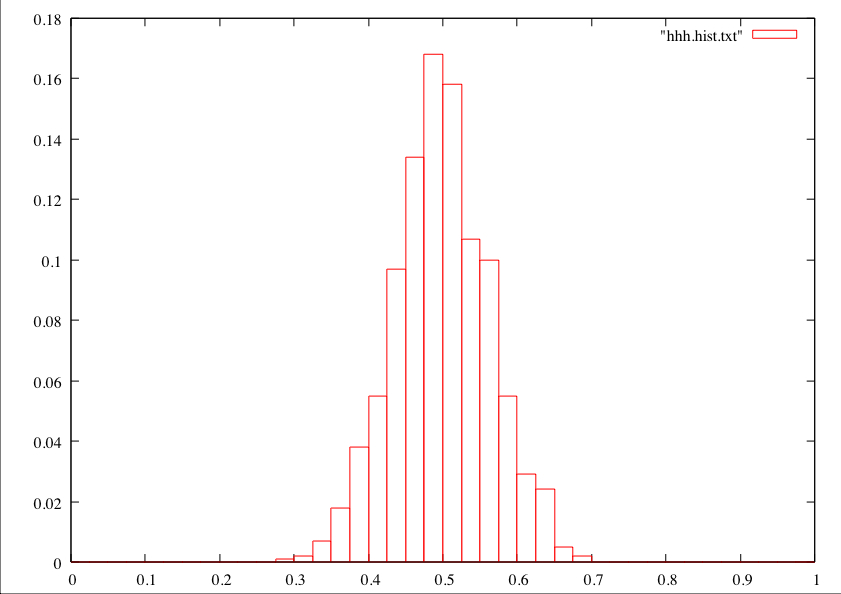
  This example bears out both of my above points. First, the "spread" got a lot smaller when more values were averaged to create sample means. Second, the shape got more like a normal distribution, with the characteristic inflection point. In general, if you are using a sample to estimate a population mean, your sample size is at least 30 or so, and there's not some obvious weirdness to the way the data looks (multiple "clumps" or wild asymmetry), you can basically just assume that you started with a normal distribution, because the sample mean distribution is going to be "normal enough" anyway.

  The next issue is that in general you don't know the standard deviation of a population ahead of time. The natural thing would be to say, "Since I don't know the standard deviation of the whole population, I will use the best estimate I have for it, namely the standard deviation of my little sample." In fact, that almost works, as we'll see shortly. For now, let's imagine that it does, and we'll attack the problem of determining the mean height of male UCSB students based on some actual numbers.

  Accordingly, suppose we take a sample of 14 UCSB students at random (the "random" part is actually tricky, by the way; how would you make sure your sample was random??), and we measure their heights, in inches, to be 70.0, 69.7, 67.3, 69.1, 65.8, 70.7, 69.5, 68.5, 67.0, 70.7, 72.1, 69.9 66.3, and 69.3. The sample mean x comes out to almost exactly 69 inches; if only we knew the standard deviation of the population, we could pull a trick like the one we did above and state some stuff confidently. So let's estimate it with the sample standard deviation, which we denote by s. Recall from above that standard deviation is a measure of how "spread out" the data tend to be away from the mean. To find s, then, take each measurement, subtract the mean, and square the difference. (Among other things, squaring makes sure that all distance, above or below, counts positively, which is good, right? We don't want large positive and negative differences canceling out if we want to measure how spread out the data are.) We then add up these squares, divide by one less than the number of data points, and take the square root. (I know, I know, it would make a lot more sense to divide by the number of data points, so you were just averaging. There's actually some controversy in the world of statistics which number you should use to divide by when you calculate the thing called the "sample standard deviation;" the reason I made the choice I did will be spelled out in the next section.) If you like things in formulas, well, here you go:
  s² = (&sum (x_i − x)²)⁄(n − 1),
  where the subscript "i" is used as a label for the data points (so x₁ = 70.0, x₂ = 69.7, etc.), &sum means to add 'em all up, and n is the number of things in your sample. (s² is called the "sample variance," which it turns out will come in handy as well.) Now take the square root of that to find s. I got s &asymp &radic42⁄13 &asymp 1.80 when I did this. So if we decide that the sample standard deviation 1.80 is a good estimate for the true population standard deviation, then we can assert with 95% confidence that the true population mean is somewhere in the range 69.0 plus or minus our magic number 1.96 times 1.80⁄&radic14, which is about 69.0 ± .94. Thus we are 95% confident that the mean height for UCSB male students is between about 68.06 and 69.94 inches.

  Getting it Right to a t

  As I mentioned above, the method used in the last example is almost, but not exactly, correct. The slight incorrectness is due to the error that got introduced when we used the sample standard deviation s as a direct substitute for the true population standard devitaion &sigma. A guy about a century ago named Gosset figured out that you need to use a different distribution from the normal in order to make up for this error, and in fact the specific distribution you need depends on your sample size. The various distributions are called Student's t-distributions, named after Gosset, who had to publish under a pseudonym due to some contractual wackiness with his employer, Guinness Stout. (Yes, it's true - like I could make that story up!) The various t-distributions are shaped roughly like the normal, but they are a little wider, to allow for more error. Here is a nice table of values, similar to the one found in the normal table link above, except that it can't be as detailed because there are so many different distributions! The &infin row in this table is the ordinary normal; notice that as you go down the row, the numbers get closer and closer to the normal values. In order to calculate with our friend Mr. t: use the row in the t-table for (n−1) degrees of freedom. (The concept of degrees of freedom is some statistical mojo that we don't have to worry too much about -- at least for now.)

  Finally: the right height! OK, now let's at long last work out the correct answer to the problem of determining, with 95% confidence, the mean height of a male UCSB student based on our random sample of 14 students. We first calculate
  s &asymp &radic42⁄13 &asymp 1.80,
  divide by the square root of the sample size to get 1.80⁄&radic14 &asymp 0.48 and then look in the row of the t-table for 13 degrees of freedom. For 95% confidence, we use the 0.025 column (aren't you glad you spent that time way back when acquainting yourself with the normal table??), which gives 2.160; so we are in fact 95% confident that the mean height for all male UCSB students is somewhere in the range
  69.0 ± 2.160 &sdot 0.48 &asymp 69.0 ± 1.03 = [67.97,70.03].

  This range is called a 95% confidence interval for the mean. Observe that it's a little wider than the "almost correct" one we produced back before we met Student. (Based on the formulas used, can you spot the reason why it's wider?) The notion of confidence is a very useful one in statistics, so make sure you understand what this statement says.

  Discussion Question: Imagine a 90% confidence interval for the mean, based on the same info. Would it be wider or narrower? Why? Exercise: Go ahead and calculate that 90% confidence interval, and use your answer to check your response to the above Discussion Question. Make sure you can answer the "Why?" part, even if you got it wrong the first time! (Answer: About [68.15,69.85].)

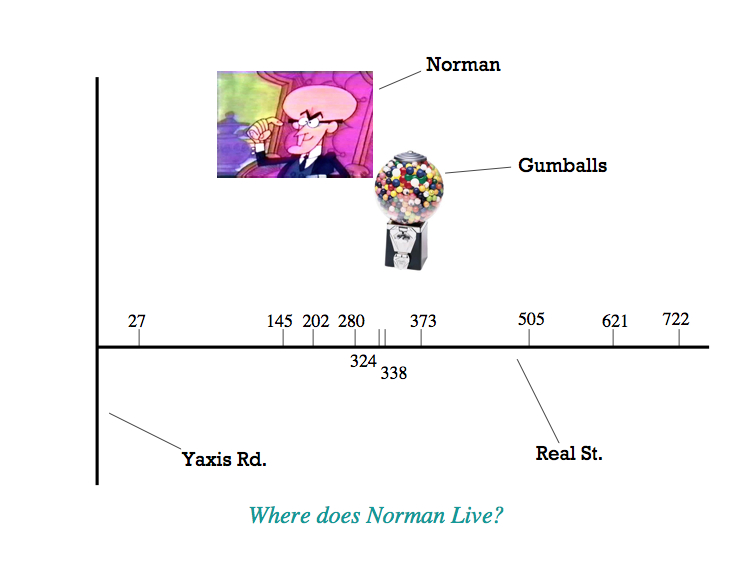
  Problem: "Normal Norman" is the FBI's nickname for a bubble-gum thief who operates entirely on Real Street, a long straight street whose addresses measure the distance, in hundredths of miles, from the point where the street dead-ends into Yaxis Road. We know from a large database of serial bubble-gum thieves that they tend to strike in a pattern that is normally distributed about their home. There have been thefts fitting Norman's pattern near the following addresses along Real Street: 27, 145, 202, 280, 324, 338, 373, 505, 621, and 722. The FBI wants you to find a 90% "hot zone" for Norman's residence; in other words, they want you to come up with a range of addresses within which you're "90% sure" that Norman lives. Can you find the desired "hot zone" and thus help them end this crime spree?

  

  ---

  The Plane Truth About Bivariate Normals

  We've managed to solve a problem fairly analogous to the one we're actually interested in solving, but in only one dimension, so our task now is to translate all of our newfound knowledge up a dimension and into the xy-plane. The kind of distributions we'll be using for this analysis are bivariate normal distributions. As you might imagine, these distributions are more complicated than their single-variable counterparts.

  First, let's define a bivariate distribution: Imagine taking data that comes in ordered pairs; they could, for example, be (height, length of left arm) for American adult females, or they could be (x-coordinate, y-coordinate) for, oh, I don't know, a series of heinous crimes committed in Los Angeles (relative to a coordinate system of our choosing). The x and y variables could be independent, meaning roughly that knowing the value of one of the variables gives you no information about the values that the other variable might have, or they might not be. In the first example of this paragraph, height and shoe size are surely not independent, since taller people, for the most part, tend to have longer arms. Note that independence is not about guarantees, just about the distibution that one variable has once you fix a value of the other variable. Now, a bivariate normal distribution is defined in terms of formulas, which I don't want to worry about too much for this course, but you can kind of spot them if you know what you're looking for, so let's start with an example or two.

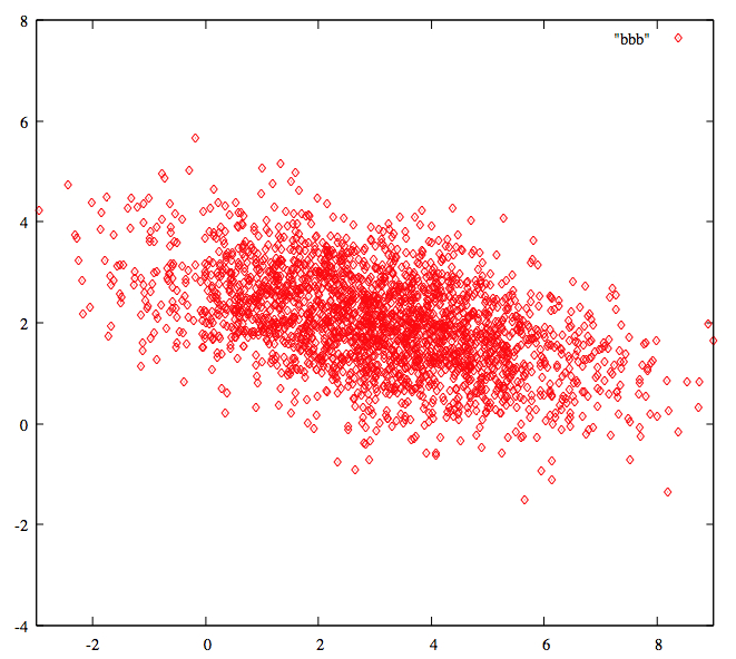
  Suppose that we took a good darts player, told her to aim at the bull's-eye, and recorded the spots she hit over a large number of throws as (x,y) coordinates measured with the bull's-eye as the origin. The "center" of her tosses would probably be very near the origin. We might also assume that her errors in the x- and y- directions are more or less independent: for instance, knowing that she was 2 inches too far to the right gives you no information about her vertical error. We might also assume that her errors in the vertical direction are generally the same size as her errors in the horizontal direction. If we plot all of these points, we may get something that looks a little like

  

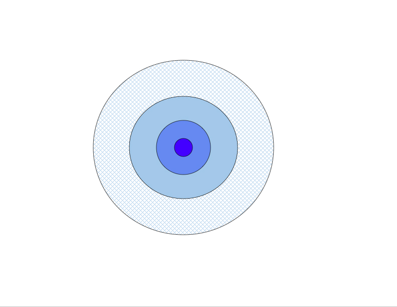
  this, where darker regions correspond to a higher density of outcomes. Notice that the data points are concentrated toward the center, just as in our friend the single-variable normal distribution, and in this case, the distribution of y-values is independent of the x-value chosen, and vice versa. The gadget corresponding the the "bell curve" in one variable would actually be 3-D and look a bit like the figure below.

  

  Now, in the "tail wagging the dog" spirit of the earlier discussion, imagine that you see the pattern of points but don't know where the bull's-eye is, and you want to come up with some region where you're 95% confident that the bull's-eye must live -- a 95% confidence region, if you will. The most natural shape you'd hope for would be a circle, provided we still are assuming that the x- and y- errors are independent and similar in size. (I should note that the variables might be independent and yet the pattern might not be circular; for example, if the dart thrower's vertical error was in general twice as large as her horizontal error, each circle in the figure would become an ellipse with long axis vertical and short axis horizontal. The issue of circles vs. ellipses for independent data is really just one of scaling -- choose appropriate (possibly different) units for the two variables, and it'll come out circular.)

  On the other hand, what if x and y aren't independent? A good example is seen here, where SAT scores are plotted vs. ACT scores and each point stands for an individual student.

  
  A plot like this one, where two measurements are made on a set of individuals to form a bunch of (x,y) pairs, is called a scatterplot. These are tremendously useful critters, but for our present purposes, note that for any fixed x-value, the y-values seem to be distributed in a pattern that depends on what x is. Assuming that the y's are normally distributed for each x, this will be another bivariate normal distribution, but this time the x and y are not independent. (Since the mean y measurement increases as x increases, we say that x and y are positively correlated -- but that's a topic we'll have to come back to later!) The dispersion of scores is this scatterplot is "elliptical," as opposed to the "circular" dispersion in the dart example: How "unusual" a score is depends on what direction, and not just how far, it is from the center. In this example, one might want to use the given data points to find a 95% confidence region for the mean pair of scores, by which I mean the "center of mass" of all pairs for the entire population. This mean just consists of the point where x is the mean ACT score and y is the mean SAT score, assuming bivariate normality; the natural shape for a 95% confidence region would be an ellipse inclined at an angle that matches the grouping of the points.

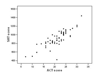
  Briefly, then, one of its salient features is that both variables are normally distributed on their own, and furthermore, if you set one variable equal to a fixed number, the possible outcomes for the other variable are normally distributed, no matter what fixed value you use. As noted above, the particular normal distribution may depend on the fixed value. For instance, the (height, arm length) pairs discussed above would likely have a distribution that is fairly close to a bivariate normal. The mean arm length would go up as the height went up, and vice versa. The next question is how to find the circles or ellipses coming from a bivariate normal distribution. With one variable, all we needed to deal with were the mean x and the standard deviation s from our sample. With a bivariate normal, we have an analogous mean (x, y), but this time instead of just a standard deviation, we need to describe the spread of both variables and also how the location of one variable affects the location of the other. Miraculously enough, this is all encoded neatly in the variance-covariance matrix for the two variables. Here's how it works: If you have a sample of n points, the covariance between x and y is calculated as

  Cov(x,y) = (&sum (x_i−x)(y_i−y))⁄(n−1) Example: Let's just run a quick calculation to make sure we're on the same page as to how this all works. Suppose we have the three data points (1,2), (2,2), and (3,8). Then it's easy to calculate x=2, y=4, so the numerator of our formula for Cov(x,y) is
  (1−2)(2−4)+(2−2)(2−4)+(3−2)(8−4)=2+0+4=6.
  Divide by n−1=2 to get Cov(x,y)=3.
  A couple of points about our new friend covariance are in order.
  • The above formula ought to look somewhat familiar! In fact, if you made the y's into x's in that formula, it's exactly the gadget we used to calculate the variance s² back in the one-variable case. So Cov(x,x) = s_x², where we subscript to distinguish which variable we're talking about now that there's more than one.
  • A glance at the formula shows that Cov(x,y) and Cov(y,x) are equal: in fact, every term in the numerator will be exactly the same in both calculations.
  We can now define the variance-covariance matrix as the 2-by-2 matrix

  Cov(x,x)	Cov(x,y)
  Cov(y,x)	Cov(y,y)

  (Please forgive my using a yellow box for "matrix notation," but I can't find a way in HTML to put the big parentheses around the table. Either someone can help me format matrices, or the convention for this class will be that matrices are yellow boxes! I will also note here that when there is only one row involved, I will occasionally use row vector notation, for example [x,y], instead of making a yellow box.) Using the above observations, we can reduce this matrix to

  sx2	Cov(x,y)
  Cov(x,y)	sy2

  In fact, an "idealized" bivariate normal has a similar variance-covariance matrix associated to it; the difference is that the numbers come from the "whole population" of points, rather than just a sample. The form of this matrix is slightly different:

  &sigmax2	Cov(X,Y)
  Cov(X,Y)	&sigmay2

  Here we use &sigma to stand for the population standard deviation and capital X and Y to reflect the population, or idealized, variables.

  With me so far? Up to this point, we have stored, rather conveniently but somewhat mysteriously, our variance-covariance information in a matrix. The convenience will become even more manifest, and some of the mystery melt away, yea, like a shroud of mist in the morning sun, before long. But first, we have to remember, or learn as the case may be, how to multiply matrices.

  First, a little notation: We call a matrix m×n, read "m by n," if it has m rows and n columns. Note that it's easy to add two m×n matrices: just add the corresponding elements in the two matrices and get the m×n matrix of sums. Subtraction is of course similar, but multiplication is a hair trickier. For one thing, if you have two matrices A and B, you can't multiply them unless the number of columns of A is the same as the number of rows of B. So let's say that A is m×n; that means B needs to be n×k for some k, or the deal's off. If this is the case, the product AB is a new matrix, the dimensions of which are m×k, and you calculate each entry in this matrix by summing the products of the corresponding elements in the appropriate row of A and the appropriate column of B. For example, suppose that

  A =

  1 2 3 4 5 6

  and B =

  7 8 9 10 11 12

  then A has three columns and B has three rows, so the two matrices can be multiplied. The resulting matrix is 2×2; as an example, to find the element in the first row and second column of AB, we use the first row of A and the second column of B, adding the products of the corresponding elements to get
  1⋅8 + 2⋅10 + 3⋅12 = 64.

  Exercise: Calculate the full matrices AB and BA. (Note that often it only makes sense to multiply matrices in one order, but the dimensions of these allow us to multiply them in either order.)

  Answers:

  AB =

  58 64 139 154

  ;  BA =

  39 54 69 49 68 87 59 82 105

  Don't even try to tell me that wasn't a good time. Now it's time for a few Fun Facts about matrices:

  • The m×n zero matrix, written 0_m×n is, not surprisingly, the m×n matrix full of zeroes. It has the nice (and obvious) property that, if A is any m×n matrix,
    A + 0_m×n = A = 0_m×n + A. It's also pretty clear that, as long as it's "legal" to do the multiplication, 0_m×n times any matrix results in a (possibly different-sized) 0 matrix, since every single multiplication you do to calculate the product is 0.
  • A square n×n matrix with 1s on the diagonal going from top left to bottom right and 0s everywhere else is called the n×n identity matrix, or I_n for short. I_n has the fun property that if you multiply it on either side by any "legal" matrix, the product is that matrix. I think you'll see why if you just multiply out

    1 0 0 1

    a b c d

    and

    a b c d

    1 0 0 1

    on your own. (Come on, do it! It takes about 30 seconds. There. See?)
  • The inverse of a square n×n matrix A is the n×n matrix you can multiply by A on either side and get I_n, the n×n identity matrix. The notation for the inverse of A is A⁻¹. The conscientious student, by which I mean anybody who's bothered to read this far, might notice that I've done a little fudging here. First off, why should such a matrix exist?? In fact, it doesn't always exist, as you can easily see by the example of the n×n zero matrix. Nothing you can multiply by that one to get the identity! Second, couldn't there be different matrices, depending on which side you multiply? Fortunately, for a 2×2 matrix, we can work everything out directly, and that's the only matrix size we'll worry about. If we write

    A  =

    a b c d

    ,  then    A−1  =

    d⁄(ad−bc) −b⁄(ad−bc) −c⁄(ad−bc) a⁄(ad−bc)

    as long as ad − bc isn't equal to 0, of course. (If ad − bc = 0, then A has no inverse.) You can, and should, check that if you multiply the two above matrices in either order, the result is I₂.

    Now we're going to use our newfound skills on the bivariate normal. Recall that the problem we're working on is (roughly) to figure out a region containing a desired fraction of a bivariate normal population, and that in order to solve the analogous problem in one variable we looked at how many standard deviations we needed to move from the mean. The variance-covariance matrix of the bivariate normal is going to serve a similar role to the standard deviation in one variable. In fact, we're going to use the inverse of that matrix to "undo" the effects of variance and covariance and "standardize" the variables, so that we can use a single lookup table for all bivariate normal distributions, analogous to the above one-variable normal table.

    Here are the details: Call the variance-covariance matrix &Sigma. (I apologize for the apparent double use of the symbol, but both are absolutely standard! In fact, it will generally be very clear from the context whether I mean "variance-covariance matrix" or "sum." Also, they are in fact distinct characters: The variance-covariance matrix symbol (&Sigma) actually looks smaller than the sum symbol (&sum).) Then an equation of the form

    x−&mux y−&muy

    &sdot  &Sigma−1  ⋅

    x−&mux y−&muy

    =   constant

    gives an equation of degree 2 in x and y. As we may or may not remember from pre-calc or some such class, as long as the x² and y² terms are both positive, the graph of this gadget is either a circle or an ellipse. (For our purposes, these terms are always going to be positive, because the variances &sigma²_x and &sigma²_y are both positive.)

    OK, let's do an example. Suppose that we have a bivariate normal distribution with &mu_x = 3, &mu_y = 2, and variance-covariance matrix

    Σ =

    4 −1 −1 1

    and, just for yuks, choose the constant to be 5. After we work out &Sigma⁻¹, our matrix equation then becomes

    x−3 y−2

    1⁄3 1⁄3 1⁄3 4⁄3

    x−3 y−2

    =   5.

    Doing the first matrix multiply first gives

    (1⁄3)(x−3)+(1⁄3)(y−2) (1⁄3)(x−3)+(4⁄3)(y−2)

    x−3 y−2

    =   5.

    Now, do the final matrix multiply and multiply through by 3 to get (x−3)² + 2(x−3)(y−2) + 4(y−2)² = 15. I used the wonderful plotter found on this web page to generate the graph of our ellipse, which looks like so: Notice that the center of this ellipse is right at (3,2). Different constant values would change the size of the ellipse, but their shapes would be similar, their centers would all be at (3,2), and their angles of inclination would all be identical. Below is a scatterplot of randomly generated data from the same bivariate normal distribution. Notice how the shape of the points follows an elliptical pattern of the same shape, and at the same angle of inclination, as the above ellipse.
    

    Exercise: Back in the dart example, we postulated that our thrower's horizontal errors x and vertical errors y are independent of one another, meaning that their covariance is 0, and that the variances of x and y are equal. Show that the variance-covariance matrix is a multiple of I₂ and that, regardless of the chosen constant on the right-hand side, the matrix equation gives a circle.

    Of course, the constant on the right-hand side of our matrix equation tells us what proportion of the population lies inside the resulting ellipse. As I hinted at above, there is a single table of values that we can use to answer that question regardless of the specifics of the given bivariate normal distribution; the values in the table come from a &chi²₂, read as chi-squared with two degrees of freedom, distribution. Here's that table, together with directions. To be honest, the only thing I have ever seen done with a &chi² involves the "right tail," illustrated in the left-hand sketch below, and I find it a little weird that they'd even put in the left-hand extreme probabilities, but hey, they're the pros.

    
    For us, the important row is the "2 degrees of freedom" row, but in fact, there are &chi² distributions with any positive whole-number degrees of freedom; they can be used for higher-dimensional multivariate normal distributions (among other things!).

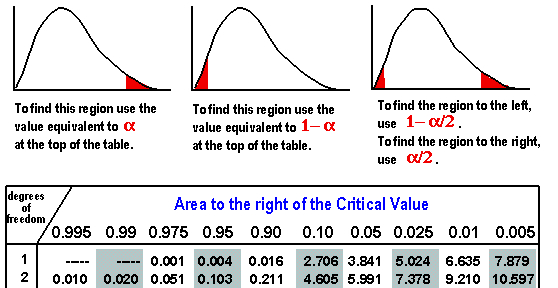
    As an example of how to use this table, the constant value 5 we used above generated an ellipse that contains between 90% and 95% of the entire population, since 90% are within the ellipse you get from using the constant 4.605 and 95% are within the ellipse coming from constant value 5.991. (Observe that we had to subtract from 1, because this table tells you how much of the population is above the given value, which means the part outside our ellipse!) If you need a more precise answer, you can use the nifty calculator found here. I plugged in 2 for "d.f." and 5 for "c²," and it gave me a "probability" value of 0.0821; in other words, .9179, or 91.79%, of the population is within our ellipse with constant value 5.
    Exercise:The calculator can calculate both ways; in other words, if you need a constant for exactly 84% of the population, it will do that for you, too. Try it. What constant did you find? (Answer: 3.665)

    Take Me to a 90% Confidence Region of Home!

    OK, I'll bet you know the last step! If the mean values and variance-covariance matrix of a bivariate normal distribution are unknown, we can generate a confidence region for the true mean (&mu_x,&mu_y) as a circle or ellipse around the sample mean (x,y). Similarly to the one-variable case, we estimate the variance-covariance matrix &Sigma with the sample variance-covariance matrix, which I'll call S. The form of our ellipse equation is thus

    n &sdot

    x−x y−y

    &sdot  S−1  ⋅

    x−x y−y

    =   constant

    Just as for the one-variable case, we have to compensate for our uncertainty about the true variances in our population by using a modified distribution in our lookup table. The factor of n reflects the fact that more data points will tighten up our confidence region. (The fact that we use n instead of √n in the formula may look as though it's at odds with the one-variable analysis, but it's due to the fact that the form of our equation changed so that the variables are all squared now, so the dimensions of our confidence region still shrink proportionally to √n. For more on this point, please see the optional section at the bottom of this page.) The distribution we use is called the F-distribution, and it requires that you specify two different degrees of freedom: the one in the so-called "numerator," which has to do with the dimension of your multivariate normal, and the one in the "denominator," reflecting the size of your sample. Since there are so gosh darn many different F-distributions, a table of values is typically unwieldy, so instead I'm just going to point you to a calculator that can help you find the confidence level associated to a specific value of the constant. The appropriate degrees of freedom to enter are 2 in the numerator and n − 2 in the denominator, where n is the sample size (number of points in your sample). Now, be careful: the value for F to plug in is your constant times (n−2)⁄(2n−2). Running the calculation then gives, as usual, the fraction of the time the true mean will live outside your ellipse. Notice that the calculator runs the opposite direction to how you might want it to; if, say, you want to find a 95% confidence region, you have to play around with constants until the calculator spits out a "p" value of .05.

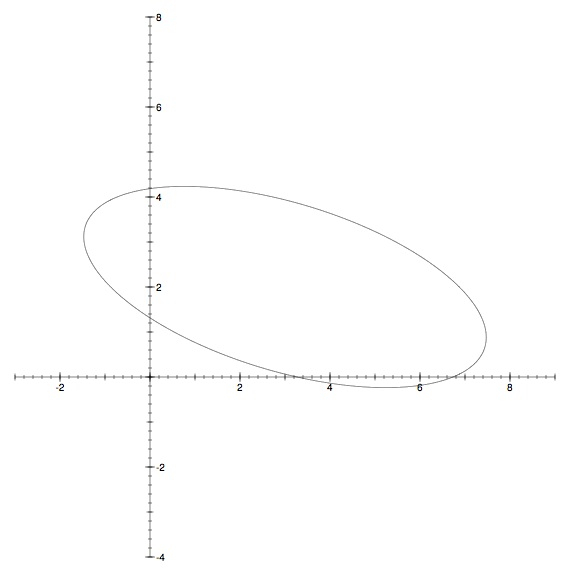
    For example, suppose that we've estimated our variance-covariance matrix using a sample of 23 points. Then we use 2 degrees of freedom in the numerator and 21 in the denominator. To find the appropriate constant for 90% confidence, I played around until I got "p" to equal 0.1, which I found for F = 2.5746. Then I multiplied this by 44⁄21 and got the constant value 5.3944 for 90% confidence. If I then wanted to graph this 90% confidence region, I would use the estimated variance-covariance matrix from the sample, the sample means, and the above formula with n=23, and toss all that info to our equation-plotting friend we met earlier.

    Optional: Nuts and Bolts

    We are now in a position to dig a little bit deeper and really understand what's going on with all this variance-covariance stuff. It's cool enough that I personally believe it will keep your interest, and the ideas are certainly important if you're going to do any serious work with multivariate distributions, but I can't lie to you and say that it's absolutely essential to know the details of this section in order to do the manipulations for this course.

    A bivariate normal distribution can be defined as any distribution arising as a linear transformation of a distribution consisting of two independent standard normal variables, plus a constant vector. (Recall that standard in this context means &mu = 0 and &sigma = 1.) In other words, if U and V are independent standard normal variables, and A is a 2×2 matrix, then the matrix product [U,V]A + [&mu_X,&mu_Y] results in a vector [X,Y] that has a bivariate normal distribution, and conversely, any bivariate normal distribution arises in this way. The mean of this distribution is [&mu_X,&mu_Y], and we can figure out the variance-covariance matrix for X and Y from the coefficients of A, but to do that we'll need to make a few observations about how variances and covariances work.

    First, if we multiply all the x-coordinates by a constant, say c, what happens to the covariance? In other words, if we know Cov(x,y), can we calculate Cov(cx,y)? Well, first off, if you multiply all the x_i by c, then the average gets multiplied by c as well, so the mean of our new values is just cx. Now, let's throw that info into the above formula for covariance to get

    Cov(cx,y) = (&sum (cx_i−cx)(y_i−y))⁄(n−1) The c factors right out, and what's left is the expression for Cov(x,y). Thus we see that Cov(cx,y) = c &sdot Cov(x,y). The second issue to tackle is the covariance of a sum. Suppose that we have a bunch of (x,y) pairs and a bunch of (z,y) pairs, and that we know the covariance for each. Now, suppose that we form the sum x + z of variables, so we can consider pairs (x+z,y). Since the mean of the sums x_i+z_i is pretty obviously x+z, the covariance formula becomes Cov(x+z,y) = (&sum [(x_i+z_i)−(x+z)] (y_i−y))⁄(n−1). Now, clearly (x_i+z_i) − (x+z) = (x_i−x) + (z_i− z), so by the distributive law, the sum splits apart into the expression for Cov(x,y) plus the expression for Cov(z,y). In other words, Cov(x+z,y) = Cov(x,y) + Cov(z,y).

    Finally, it almost goes without saying that the covariance of anything with a constant is 0: if the x_i are all equal, then they are all equal to x, and every term in the sum would involve a factor of x_i − x = 0. In light of the above facts, then, the variance-covariance matrix of X and Y is the same as that of X − &mu_X and Y − &mu_Y, which we can calculate as follows. If we write

    A =

    a b c d

    ,  then

    X − &muX Y − &muY

    =

    U V

    &sdot A =

    aU+cV bU+dV

    One important technical point is that we insist that ad − bc &ne 0, because otherwise X and Y would be constant multiples of one another. As noted above, this means that A has an inverse. Since U and V are standard and independent, &sigma_U² = &sigma_V² = 1, and Cov(U,V) = 0. Therefore, we can use the formulas for sums and multiples we worked so hard to obtain, and we calculate the variance-covariance matrix &Sigma of X and Y as

    a2+c2	ab+cd
    ab+cd	b2+d2

    
    Recall that the transpose of an n×k matrix Mis the k×n matrix M^T obtained from M by making the rows into columns and vice versa. The important property of transposes is that (MN)^T = N^T M^T. This property is not as mysterious as it looks at first: The point is that the multiplication you do for each element in the transposes is exactly the same as the one you originally did on the untransposed matrices, but with rows and columns switched around. (Work out a small example, say 2×2, and you'll see how it works.) As you should now check, the &Sigma we calculated above is equal to A^TA. Therefore

    U V

    =

    X−&muX Y−&muY

    &sdot A−1.

    Using properties of transpose, it is easy to show that (A^T)⁻¹ = (A⁻¹)^T: Just multiply out A^T (A⁻¹)^T = (A⁻¹ A)^T = I^T = I. So &Sigma⁻¹ = A⁻¹(A⁻¹)^T, and we can put this all together and calculate that [X−&mu_X,Y−&mu_Y]&Sigma⁻¹[X−&mu_X,Y−&mu_Y]^T = [X−&mu_X,Y−&mu_Y]A⁻¹(A⁻¹)^T[X−&mu_X,Y−&mu_Y]^T    (from substituting in the above expression for &Sigma⁻¹) = [X−&mu_X,Y−&mu_Y]A⁻¹ &sdot ([X−&mu_X,Y−&mu_Y]A⁻¹)^T     (by the abovementioned property of the transpose of a product) = [U,V] [U,V]^T = U² + V². Now, the &chi² distribution with r degrees of freedom is defined as the sum of the squares of r independent standard normal variables, which is exactly what U² + V² is in our case r = 2, so we see where the specific matrix &Sigma⁻¹ comes into the picture - namely, it's exactly the matrix you need to use in order to "undo" the given distribution into independent standard normals, due to the factorization &Sigma⁻¹ = A⁻¹(A⁻¹)^T. We also see why the &chi² is the appropriate distribution to use to find the constant values: it just came out of the way we "standardized" our variables.

    This general method works for any number of variables you like. For example, we could have done all of this in one variable as well, and the answers would have come out just the same as they did in the first part of this lesson when we were dealing with single-varaible normal distributions. Let's check that claim: In one variable (start out with known σ), the variance-covariance matrix has only one entry, namely &sigma², and the equation for the boundary of our confidence region becomes simply (x−&mu) &sdot (&sigma²)⁻¹ &sdot (x−&mu) = const, or (x−&mu)/&sigma = ± √const, or x = &mu ± &sigma √const. The constant here is governed by a &chi² distribution with one degree of freedom, which is just the square of a standard normal distribution, hence the square root on the constant. Finally, here are a few details about the changes you have to make when doing confidence intervals, which are really just 1-dimensional confidence regions. First off, the an F-distribution with 1 degree of freedom in the numerator and k in the denominator, which is what we'd use for (k + 1) one-dimensional data points, is the square of a -distribution with k degrees of freedom, which is the distribution we discussed way back when. √n comes from the fact that we need to take the square root of both sides, just as when we went from &chi² to normal a few lines up. (The correction factor (n−2)⁄(2n−2) we needed to multiply by our critical F-value becomes, in one dimension, (n−1)⁄(1n−1) = 1.)