CS190N
Numb3rs -- Sacrifice
The situation:
Charlie is able to observe, through the miracle of "van Eck
phreaking," the rhythm of the keystrokes used by a killer to login to
his victim's computer and subsequently erase the data from its hard
drive (see those 0s and 1s on the screen?). By matching this rhythm
with the password-entry rhythms of a known user, he is able to
identify that user as the killer. How did he do it? What do those
horizontal bars mean? Will it hold up in court? Most importantly,
after Don clearly understood what Charlie was talking about, why did
Charlie feel compelled to launch into that whole thing about concert
pianists? Stay tuned for the answers to precisely none of the above
questions; instead, we will take a look at some better questions,
their answers, and a lot of information about information.
Speaking Hypothetically
In the first unit, we encountered the notion of a confidence
region as a means of quantifying the information obtained through
a random sample. In fact, there is another concept in statistical
inference that is related and equally important as, but distinct from,
the confidence region &mdash the Castor to its Pollux if I may,
the Mary Kate to its Ashley if you will &mdash namely, the
hypothesis test. As my beloved audience seems to have
encountered ideas in this space before, I will give a brief but
meaningful resumé of the simplest examples of these things.
Hypothesis tests differ from confidence regions in their goals: Rather than
trying to estimate a parameter, with some measure of certainty, a test
attempts to answer a yes-no question, again with a measure, quantified
in a very specific way, about the certainty of the answer. The
question typically involves the equality of a population parameter,
such as the mean, either to a constant or to the corresponding
parameter of a second population. For example, we may wish to test
whether the mean height of all male UCSB students is
5′10″, based on a sample, or we may wish to test whether
there are differences in the mean response of patients to two
different drugs. I could go on all day with examples of how
statistical tests can be used in the real world.
The most straightforward examples of hypothesis tests involve the question of
whether a population mean is equal to a given constant
&mu0. The statement that they are equal is called the null
hypothesis and is written out formally like so:
(H0 is pronounced "aitch null.") Against the null
hypothesis, we present an alternative hypothesis, written
Ha, which in this
example can take one of three forms, depending on what specific
question we're interested in answering:
Ha:
&mu &ne &mu0 or
&mu < &mu0 or
&mu > &mu0
| |
|
(For the sake of simplicity, let's continue the present discussion
assuming that the alternative hypothesis of interest is the "&ne"
version.) Having set up our opposing hypotheses, we then move
along to taking a sample and evaluate, in a way that will be discussed
in our usual painful detail below, the two hypotheses relative to the
data.
Note the asymmetry in the two hypotheses: they are not
interchangeable. Our null hypothesis &mdash and this is absolutely
typical of null hypotheses in general &mdash is too specific to be
literally true. I mean, if we return back to the example of the
UCSB males, it's pretty clear that if we had enough precision in our
measuring instruments and used this precision in recording our
measurements, the mean height would have (essentially) no chance of
being exactly 5′10″. So what's all this hypothesis-testing
business about, anyway? Why couldn't we just answer any null
hypothesis involving an "equal" sign with "Uh, no, like, what are the
chances? Please!" before even taking a sample, and then spending all
the time and grant money we saved on a really good sandwich?
The fact of the matter is that you can ask, and answer, many
interesting questions that don't involve the numerical precision of
the null hypothesis. Often, for instance, the null hypothesis is
something we posit skeptically, defying the sample to provide really
good evidence against it. I'll give you an example: Suppose that we
know from a bunch of evidence that the average cold sufferer takes
just about 4 days to get over the cold. Little Giant Pharmaceuticals
releases a product that it claims will reduce the amount of recovery
time. Let's posit that their product had no effect and
consider the times-to-recovery from a cold as our population. We
set up the null hypothesis H0: &mu = 4 and sit
back and wait for the (sample-based) evidence. Now, if they were to
come back and say, "We gave it to three cold sufferers and, on
average, they took only 3.6 days to get over their colds!" we would have
cause to doubt whether the product made any difference at all; in other
words, that kind of data is not all that out of whack from our assumed
value of 4 for the mean. On the other hand, if they did a responsible
clinical trial and found that, among 472 cold sufferers, the mean time
to recovery was 1.9 days, well, we might sit up and take notice. All
this even though, really, what are the chances in either case
that the mean time to recovery for people receiving the treatment was
exactly 4 days &mdash or even exactly equal to the mean for the
population at large? Nil, that's what they are. Heck, how can we even
know the mean for the population at large in a situation like
this one? And yet we still might like to use the data in order to say
something meaningful about the impact of the treatment on the duration
of colds.
What's going on is that, just as we state the two hypotheses in
an inherently asymmetric way, we also treat them
asymmetrically. It's kind of skepticism vs. cynicism: The null
hypothesis is set up to assume skeptically that there is "no
difference," "no change," "no effect," and
is what we will assume to be true unless the sample data provide
convincing (this notion of "convincing" is adjustable, as we'll see)
evidence that it is false. This evidence will come in the form of an
analysis of how likely it would be to gather the evidence we
did, cynically assuming H0 to be true.
Now we're beginning to see how the details of a hypothesis test
look. Let's go through a specific example to see all the moving parts:
Example: Suppose that it is known that all college-age males in
the country have a mean height of 5′10″ with a standard
deviation of 2&Prime. You wonder whether there's any difference in
mean height between male UCSB students and those in the rest of the
country. Let's suppose for simplicity's sake that you are happy to
assume that the UCSB students' heights are normally distributed with
unknown mean &mu but with known standard deviation &sigma = 2. Your
hypotheses are then
H0: &mu = 70
Ha: &mu &ne 70
|
and off you go to find yourself a random sample. You measure the
heights of 16 students and find that their mean height was 70.9
inches. What do you make of this data? 70.9 is different from 70, but
on the other hand it's not different by a huge amount, but on the
other other hand the mean of a decent-sized sample should be pretty
darn close to the population mean, but on the other other other hand
is 16 big "decent-sized"? is 0.9 not "pretty darn close"? Before we run
out of hands, let's do some math, shall we? Given our assumptions, and
assuming that H0 is true, the sample means for
random samples of size 16 should be normally distributed with mean 70
and standard deviation 2⁄√16 = 0.5.
Under this set of assumptions, then, our particular sample mean lives
here in the distribution of all possible sample means:
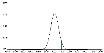
To understand how "unusual" this sample is, we should look at the
probability that a sample mean would be at least that far away
from the true mean (assuming, all along, that H0 is
true). That's the white region in the graph below &mdash sorry,
I couldn't figure out how to make the applet I scared up reverse the
colors &mdash and is called the p-value associated to this sample for
this test.
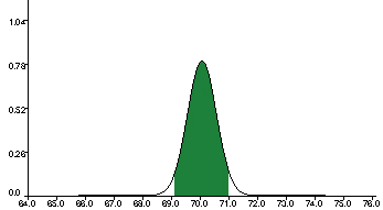
The white represents the region at least 1.8 standard
deviations away from the mean. How much white area is there? Here is
the least annoying normal table I could find in 30 seconds of online
hunting about; it shows that .0359 of the population lives at least
1.8 standard deviations to the right of the mean, and an equal amount
lives at least 1.8 to the left, so all told, about 7.18% of the
population is in the white zone &mdash, that is, the p-value in
this case is p &asymp .0718. This means that, assuming for the
moment that the mean really is 70, if you took a bunch
of random samples of size 16, about 7.2%, or about 1 in 14, would have
a sample mean at least as far away from 70 as this one is. What does
this tell us about the population mean?
This brings us to the concept of significance. Besides setting
up our hypotheses, we need to decide, before taking our sample,
how small the p-value, which represents that "outside" fraction
of the population needs to be before we'll go ahead and reject
H0 in favor of Ha. This
threshold is called the significance level of the test, denoted
by &alpha. In other words, we say ahead of time, "We'll take a sample,
measure its p-value, and reject the null hypothesis if p <
&alpha." I hope it's clear by how things are set up that the smaller
&alpha is, the more certain
we need to be that the the null hypothesis is incorrect before
rejecting it: The significance level &alpha represents the fraction
of the time that you are willing to reject H0
incorrectly. You realize, of course, that it's folly to say,
"Hey, I never want to reject H0 incorrectly!"
The only way to be sure you'll never reject it incorrectly is never to
reject it, and that isn't a very productive use of your data. A
standard value for significance is &alpha = .05, just as 95% is
standard for a confidence interval. Note how much this
privileges the null hypothesis: We don't want to reject it
unless we see evidence extreme enough to be in the rarest 5% if it
were true. Also note that lower values of α, while they make it
less likely that you reject a true null hypothesis, they also make it
more difficult to reject a null hypothesis that is substantially
false. Bearing this tradeoff in mind, and analogously again to the
situation we encountered with confidence intervals, we
can use various values of &alpha, depending on what we need to
accomplish, the real-life consequences of rejecting a true
H0, and the consequences of retaining a null
hypothesis that does not accurately model reality. In the current
example, if we have proposed &alpha = .05
for the significance level of interest, then we cannot reject
the null hypothesis, because the p-value .0718 is larger than
&alpha. On the other hand, we could reject the null hypothesis at a
significance level of .1.
There are a couple of other parallels between significance and
confidence that we ought to recognize. First, significance, like
confidence, is similar in form to probability, but
it is not probability! For instance, it makes no sense in this example
to say "There's a 7.2% probability that H0 is true."
H0 is not a random event &mdash it's either true or
it's false, and no random sample can change which of those it is. Second, level
of significance has a direct relationship with confidence level, at
least in this simple example. Namely, for a given sample we reject
H0 in favor of a two-sided alternative at
significance level &alpha precisely when the
proposed mean &mu0 lies outside the
(1−&alpha) confidence interval for the mean produced by
our sample. Another nifty way of saying the same thing is that
a level-C confidence interval consists of all the null hypothesis
values that you can't reject at significance level (1−C).
Let's talk for a moment about the other two possibilities for
Ha, the so-called one-sided
alternatives. Such an alternative could have arisen in this example
with a very small change in wording: Suppose that instead of wondering
whether the average UCSB male student is different from the
national average, you wondered whether the average UCSB student is
taller than the national average. Our alternative hypothesis
would become
Ha: &mu > 70,
and in order to answer the question we're asking, we need to measure
how unusually large our sample mean is: We would clearly never
reject the null in favor of the alternative if we got a sample mean
that was way below 70. For the specific situation we set up,
with a sample size of 16 and sample mean of 70.9, the p-value
is the probability of seeing a sample mean that large or larger when
H0 is true, is only .0359, so we can reject the null
hypothesis in favor of the alternative at the &alpha=.05 level. In
general, only those outcomes supporting the alternative hypothesis
can contribute to the p-value.
There is a connection to confidence intervals with one-sided test as
well, but this time the interval is infinite on one side, and
rejection of the null at significance level &alpha happens when the
mean proposed in H0 lies outside the
(1−&alpha) lower (as in our case) or upper confidence
bound for the mean.
A tidy way to do the calculations is to identify the test
statistic, in this case the normalized z-value, under
H0, of the sample mean, namely (X &minus
&mu0)⁄(σ⁄√n) and to
determine whether this test statistic exceeds (positively or
negatively or either one, depending on the nature of the alternative
hypothesis) the critical value for the test at the significance
level chosen.
The above example, while it's a little bit simplified, contains most
of the ingredients to the usual normality-based approach to hypothesis
testing. Now, let's have a careful look at the problem we're actually
trying to solve. When you did your typing assignments, we measured
the time intervals between each pair of keystrokes and gathered data
about particular letter combinations. For example, in the Marhta
Stewart article there are a lot of "th" strings, so we now have pretty
good information on the speed at which each of you (who completed the
assignment) tends to type "th." We propose to use data like this in
order to ascertain whether two samples were typed by the same
person. Can we set this up as a hypothesis test? We
might hope to distinguish two typists merely by the mean speed
with which they type their various letter combinations. Suppose then
that we're given two typing samples, which I will label with the very
imaginative scheme Sample 1 and Sample 2. The null hypothesis of "no
difference" would look a little like
| &muaa,1 | = | &muaa,2
|
| &muab,1 | = | &muab,2
|
| | .
.
. |
|
| &muzz,1 | = | &muzz,2
|
in other words, the mean values for each sequential letter combination
are equal between the two "populations" from which the samples were
drawn; the alternative would simply be that the null is false, since
even one mean that was truly different would indicate two different
typists. In the best possible case, we would be able to reject the
null hypothesis when the samples came from different typists and would
retain it whenever they came from the same typist. (In theory, there
are 676 equations describing the null hypothesis if we limit ourselves
only to combinations of small letters! In practice, of course, things
like "qp" and "jb" don't occur, and combinatins such as "bv" are
pretty rare.)
I hope that it's clear that this particular hypothetical hypothesis
test differs in substantial ways from the above example. First of all,
we have no precise knowledge about any of the standard
deviations. Thus, even a stripped-down version of the above in which
we examine the mean speed for a single keystroke pair of a single
typist against a specific value, say 300 milliseconds, so that our
hypotheses are
H0: &muth = 300
Ha: &muth &ne 300
|
already represents a departure from what we discussed. The extra
complication is not huge, however, provided that our data looks
reasonably normal or we have a sample size that's big enough (30 or so).
Just as in the case of confidence intervals, the process is very
similar to that for the problem with known variance, except that the
standard deviation &sigma needs to be estimated by the sample standard
deviation s, as we calculated it way back in the here,
with (n−1) degrees of freedom, where, as usual, n
is the sample size.
The next departure is that we really want to compare the means from
different samples to each other rather than comparing the mean from a
single sample to a constant. This is also a very
natural thing to do that has all kinds of real-world instantiations:
for example, a researcher may wish to see whether a particular drug
lowers blood cholesterol, on average, more than a placebo or than some
existing treatment. To look at another simplified version of our
problem, suppose that we want to see whether the "th" speeds of the
typist(s) from which two samples come are different. We would then set
up the hypotheses
H0: &muth,1 = &muth,2
Ha: &muth,1 &ne &muth,2
|
As usual, we make the formal assumption that both populations are
normally distributed, with the usual observation that this assumption
becomes less important with larger samples, and if we also make the
assumption that the standard deviations of the populations are
equal, then the test statistic looks like
|
x1 &minus
x2
|
|
|
√[(n1s12 +
n2s22)&frasl(n1 + n2 −
2) &sdot (1&frasln1 +
1&frasln2)]
|
(that radical sign covers the entire denominator!), and the critical
value is taken from a t-distribution with (n1
+ n2 &minus 2) degrees of freedom. (In the above
formula, all the means, standard deviations, and sample sizes come
from the "th" values of the appropriately subscripted typist.)
Let's examine the test statistic for a minute. The numerator is not too
unexpected: you'd want it to depend in a very direct way on how
different the two sample means are. The first factor in the
denominator is a weighted average of the variances, and the second
factor reflects the idea that sample variance decreases as the
square root of the sample size.
In fact, the above method is very sensitive to the assumption that the
standard deviations are equal. Unlike most assumptions about
distribution in this space, it's not enough to size up the two samples
and say, "Yeah, the spread looks just about the same." You should have
a good reason to believe ahead of time that the two populations
have the same standard deviation before you undertake a test using
this method; if they do not, in particular, there is a real chance
that your significance level is not accurate, meaning that you would
incorrectly reject the null hypothesis the wrong fraction of the
time. If you don't have a good reason to believe that the standard
deviations are equal, instead use the test statistic
|
x1 &minus x2
|
|
|
&radic(s12⁄n1
+
s22⁄n2)
|
against a critical value from the t-distribution with
min(n1, n2) degrees of
freedom. Many authors advise us to stay away from the previous test
entirely and always use this one, due to its aforementioned
sensitivity to the assumptions. The drawback to this test is that it
is more conservative than the previous one, in the sense that
it rejects the null hypothesis less often: Even though the test
statistic is a tad bigger, the number of degrees of freedom is much
smaller, so the critical value is correspondingly quite a bit
larger. (If that business about degrees of freedom doesn't make sense,
stare at that t-table to which I linked you above and think
about what t-distributions are all about.)
Well, this still doesn't quite give us a method for attacking the
problem posed, but we're getting there. One method that might look
attractive on the surface goes a little like this: Let's do
t-tests for each letter pair separately, rejecting that big
null hypothesis if we reject any of the simple ones. A minute's
reflection will show, I believe, that this won't quite work. Let's
suppose that we choose &alpha = .05 as our significance level, and
let's suppose that there are 100 letter pairs that actually occur in
the typing samples. Since each individual t-test has a 5%
chance of rejecting a true null hypothesis, and we're doing 100 such
tests, we're almost certain to reject our H0, even
if it's true! (In fact, the probability of rejecting a true null can
be calculated in the usual way &mdash I hope you could all reproduce
this if you had to &mdash as 1 &minus .95100 &asymp .996.)
We'll speak later of ways to improve this general approach to the
problem. Meanwhile, let's look at a couple of other common tests and
how they relate to our problem.
Chi-square (&chi2) test You (may) have actually
seen a test for carrying out multiple comparisons similar to the ones
we see here, namely the &chi2 test for equal distributions
of categorical
data. It's actually possible to extend the &chi2 test to
continuous data. One does this by (somewhat arbitrarily) making
bins comprising ranges of the data and then, for each
measurement, converting its numerical value into the label of the bin
into which it would fall. In our situation, we might take all of the
keystroke pairs in consideration between two typing samples, pool all
of the measurements together, order them, and break the range of
measurements into five bins, labeled A through E, with
20% of the data in each bin. We could then make counts of how many of
each keystroke pair for each typist fell into each of the bins,
obtaining counts caaA,1,
caa,A,2, caa,B,1, ... Our null
hypothesis should express that the
proportions of the keystroke pairs over the bins are independent of
the typist who produced them; in short (sort of)
H0: The compound variable (keystroke pair,
bin) is independent of the typist variable.
Ha: H0 is false.
|
To test this, one forms a contingency table, which in this case
would be very tall and thin:
| caa,A,1 | caa,A,2
|
| caa,B,1 | caa,B,2
|
.
.
. | .
.
.
|
| czz,E,1 | czz,E,2
|
For contingency tables such as this one, it is of interest to form the
marginal totals for each row, written ci+ =
&sumj cij, and for each column,
namely c+j = &sumi
cij. If the variables were independent, then
the proportion of things in the i, j cell, which is equal to
cij ⁄n (where n is the total number of
things in all the cells) should be equal to the proportion in the
ith row times the proportion in the
jth column, that is, ci+ ⁄n &sdot c+j ⁄n. This says that
cij should be about equal to ci+ c+j
⁄n. Accordingly, we call this last value
the expected count for cell (i, j); note that the
expected count for a cell need not be an integer! Our test statistic
measures how far off this is from being true; since errors in either
direction are evidence for our alternative against our null, it's
fairly natural to imagine that they'd be squared values; also, the
differences should be measured relative to how big we expect them to
be; for example, if your expected cell count is 400 and there are 390
in that cell, that's probably not as big a deal as expecting 15 and
seeing 5. Bearing all this in mind, I hope you're not too surprised at
the form of our test statistic:
| &chi2 = &sum&sumi, j
|
[cij &minus (ci+
c+j
⁄n)]2
|
| ci+
c+j
⁄n
|
|
Believe it or not, under H0, the statistic
&chi2 has asymptotic distribution &chi2, with
degrees of freedom equal to (# of rows &minus 1)⋅(# of columns
&minus 1). In our case, this would be 675, at least in principle. As a
practical matter, the asymptotic distribution is pretty good, as long
as there are relatively few cells with low expected counts. The rule
of thumb I've seen is that no cell should have expected count less
than 1 and that fewer than 20% should have expected counts less than
5. Observe that for the problem we're looking at, we have some
control over these considerations: if either of the above conditions
on expected counts is violated, we can reduce the number of bins into
which we throw our keystroke pairs; we can also reduce the number of
keystroke pairs we consider, which we'd probably end up doing for any
test! The real drawback to the &chi2 test is philosophical:
By lumping numerical data into bins, we have destroyed a lot of
information that is potentially useful; additionally, &chi2
treats the bins simply as categories and even "forgets" which bins
correspond to larger numbers than which others. Generally,
&chi2 should not be your first choice when looking at
numerical data.
ANOVA F-test What our problem is really looking to
do is to compare multiple means, and a common test that does, in fact,
compare multiple means is the so-called analysis of variance,
or ANOVA for short. Superficially, then, I think our problem looks
more like an ANOVA problem than like any of the other models we've
discussed above. The idea of ANOVA is that, given a number of discrete
categories, numbered 1 up to k, and numerical data
xij in each category i,
one can try to determine whether the populations within the categories
all have the same mean by breaking down
the total variation within the sample into the variation
within the categories and the variation between the
categories. Intuitively, if the variation between categories is much
larger than the variation within them, we would seem to have
reasonable grounds to believe that the means are not all the
same. Under the assumption that the data in each category is normally
distributed (becomes less important with increasing sample size) and
has about the same standard deviation (remains important!!), we can
form the hypotheses
H0: &mu1 = &mu2 =
&sdot&sdot&sdot = &muk
Ha: H0 is false.
|
The analysis of variance goes like this: Measure some sort of notion
of "typical" squared deviation from the mean within the
categories as s&tilde2 =
1&frasln
&sum&sumi, j (xij &minus xi)2,
and measure the overall variance of the sample as
s&tilde02 =
1&frasln
&sum&sumi, j(xij &minus x)2. Note that
the difference between these statistics is that s&tilde2
uses the sample mean within the appropriate category in each term, while
s&tilde02, representing the null hypothesis,
uses the overall sample mean for every term. One can show that under
H0, the test statistic
|
| F=
|
| (s&tilde02 &minus
s&tilde2)⁄k &minus 1
|
|
|
s&tilde2⁄n &minus k
|
|
has an F-distribution (remember those?!?) with (k &minus
1, n &minus k) degrees of freedom.
Unfortunately, a moment's inspection into what this test does shows
that it cuts the data in the wrong direction, so to speak. For
instance, we could use ANOVA to figure out whether there were
significant differences among the "th" keystroke-pair speeds for a
number of different typists, and it could also be used to measure
whether there are significant differences in the speed with which a
single typist types a number of different keystroke pairs. Without
further enhancement, however, it's hard to see how to use ANOVA for
our problem.
What do all these tests have in common,
how are they constructed and how does one construct similar tests to
perform one's own particular bidding?
A Likelihood Story
In order to understand this, we need to understand the concept of
likelihood. The big idea is to get a handle on how well a
probability model "explains" a random sample. I hope you're still
smarting from my last diatribe about how population characteristics
are not random and we therefore cannot speak of the
probability that a population parameter has a certain
value. Likelihood is a way of getting around that, in our favorite
tail-wagging-the-dog sense.
Suppose that we've decided that our population is distributed
according to some specific family (for example, normal), but one or
more of the parameters is unknown. Given a random sample, the
likelihood associated to a choice of parameters is just the
product of the probabilities of the sample elements in the case of
discrete distributions and the product of the values of the density
functions at the sample elements in the case of continuous
distributions. The likelihood function is thus a function of the
parameter(s), given some sample data, while the probability or
probabiliy density function is a function of the value that the
variable can take on, but they're the same function! I'll call
probability or density functions ƒ(x), typically,
and likelihood functions L, or L(&theta), or even
L(&theta | S) if I want to emphasize the sample S
on which I based the likelihood calculation.
Let's do a fairly simple example. Suppose we have a coin with p
= P(heads) unknown. We toss the coin four times, and our sample
S consists of three
heads and one tail. The value of .5 for p has likelihood
L(.5) = .54 = .0625, while L(.8) =
.83 &sdot .2 = .1024.
For a given sample, given two choices of parameter values, the one
with a higher likelihood is the one gives a higher
probability that the sample would have occurred if it were
the true parameter, and it's generally accepted that parameters of
higher likelihood are therefore "better" at explaining the
sample. Thus, in the above example, we would prefer p = .8 over
p = .5 as a model for the coin. (If this doesn't sit well with
you, I don't blame you; see the following Bayes' Rule discussion.)
Please note here that we really can't attach too
much meaning to the value of the likelihood function for a
specific value of a parameter, only its value relative to those
for other values of the parameter. In fact, two likelihoods can be
compared directly according to their ratio, due to
considerations based on Bayes' rule (again see the section below for
details).
We can also calculate likelihoods for continuous distributions, such as
the normal. For continuous distributions, of course, you need
to replace probability of an outcome with probability density at
that outcome. If this makes you a little nervous, imagine attaching a
little bit of width &Deltax onto each of the outcomes in the
sample, so that we're talking about the honest-to-goodness
probability of falling between xi and
xi + &Deltax for each element
xi in the sample. If &Deltax is small enough,
this probability is approximated well by
ƒ(xi)&Deltax; in comparing the likelihood
functions for two different values of the parameter, you would have
exactly the same number of factors of &Deltax in each
calculation, so the question of which one was bigger, and in fact
their ratio, would only depend on the densities.
When you're looking for a meaningful estimate for a parameter based on a
sample, the maximum likelihood estimator (MLE) has a number of
attractive features. First of all, ure and simple, in terms of
likelihood functions, it's the best one at explaining the data,
in the sense that there is no other value for the parameter for which
the data would have been more probable. In addition, MLEs have good
properties relative to the notion of efficiency, which is a bit
complicated for the scope of our little class, but essentially, MLEs
tend to be the "best" estimator possible in terms of mean square error
from the parameter that they are estimating.
Let's do a couple of sample calculations of MLEs. First, suppose we
toss a coin with unknown p = P(heads) n times,
and we toss k heads and (n &minus k) tails. Then the
likelihood function L(p) = pk
(1−p)n−k. To find the MLE for
p, denoted by p^ (that ^ is
supposed to be on top of the p! I love HTML!!), we need to
maximize L, which is
certainly a nice differentiable function of p between 0 and
1. It's also easy to calculate L(0) = 0 and L(1) = 0
(unless k = 0 or k = n; these cases we'll handle in a
minute), and L is a nonnegative function by its very
definition, so it has a max in there somewhere! We'll find it using
calculus. First, note that since the logarithm function is monotone
increasing, the value of p that maximizes log(L) is the
same value that maximizes L, and log(L) is easier to
handle. We calculate
log(L(p)) = k log(p) + (n−k)
log(1−p), so
d⁄dp (log L(p)) = k⁄p &minus (n−k)⁄(1−p).
To find the maximum value, we set this derivative equal to 0. When
we clear denominators we find that k(1−p) =
p(n−k), so k−kp = np−kp, and
thus p^ = k⁄n. I hope you agree that this makes
intuitive sense: our best guess for the probability of heads is the
proportion of heads in our sample.
The same result is true in the annoying "corner cases" k = 0
and k = n. In the k = n case, for example,
L(p) = pn, which is pretty clearly
maximized on the interval [0,1] at p = 1, so p^ =
1, which is still equal to k⁄n! Similarly, if k = 0, p^
= 0 = k⁄n, so we find that the same MLE formula
is valid for any sample.
Now let's try one with a continuous distribution. Suppose
that we have a random sample from a normal distribution with unknown
mean &mu and known standard deviation σ. Let's calculate
μ^, the MLE for &mu, from this sample. Recall that the density
function for a normal distribution is
ƒ(x) = 1⁄(√2&pi &sigma)
e&minus(x−&mu)2⁄
2&sigma2
so for a given sample S = {x1,
x2, ..., xn}, the likelihood
function is given as
L(&mu) = &Pii 1⁄√2&pi&sigma
e&minus(x−&mu)2⁄2&sigma2.
Clearly the log trick is in order once again! Taking the log turns the
product into a sum and gets rid of exponents:
log L(&mu) = &sumi [log(1⁄√2&pi &sigma) +
log(e&minus(xi−&mu)2⁄2&sigma2)]
= n log(1⁄√2&pi &sigma) &minus
&sumi(x−&mu)2⁄2&sigma2, so
d⁄d&mu (log L(&mu)) =
&minus&sumi(xi &minus
&mu)&frasl&sigma2
= (n&mu&minus&sumxi)&frasl&sigma2.
Setting this equal to 0 amounts to setting the numerator equal to 0,
and this gives &mu = &sum
xi⁄n = x. As this is the only
critical point, and you could surely make log L(&mu) as small
as you like by making &mu really really big, the critical point must be a
maximum, which as we said just 30 seconds ago makes it a max for
L itself. So &mu^= x. Again, this result
probably isn't too surprising: the most likely choice for the
population mean is the sample mean.
We can stretch the above example to find the MLE (&mu, &sigma) for a
normal when both parameters are unknown! The likelihood
function L(&mu, &sigma) is exactly the same symbolically as we
calculated before, but since this time &sigma is a variable, we need
to set the two
partial derivatives of log L equal to 0 in order to find
the max.
Exercise Carry out the calculation for the MLE for (&mu,
&sigma). Based on what we've seen from MLEs so far, is your answer
just exactly what you had expected?
Bayes' Rule
If you really want to understand likelihood, you need to come to grips
with Bayes' rule. I hope you've seen this in
probability class, but let's review quickly how it works. Recall
that for a given random variable, an event is a subset of the
set of all possible outcomes of the variable that has a measurable
probability (maybe 0). If A and B denote events, then
the probability that both occur, written P(A &cap
B), can be expressed as the probability that A occurs
times the probability, given that A occurs, that B also
occurs. In symbols,
P(A &cap B) = P(A) &sdot
P(B | A).
I hope this make intuitive sense: If 30% of all students on campus
have "first-year" status, and 10% of all students with "first-year" status
are business majors, then the probability that a randomly chosen
student will be a first-year business major is .3 &sdot .1 = .03. Note
that this example does not assume that being a first-year student and being a
business major are independent; thus, if you were only given the
overall percentage of business majors on campus, you would not
have enough information to do the final calculation.
Since the event A &cap B is surely the same event as
B &cap A, we can reverse the roles of the two variables
on the right-hand side of the above equation and obtain
P(A) &sdot P(B | A) =
P(B) &sdot
P(A | B);
Dividing both sides by P(A) then gives Bayes' rule in
its simplest form:
P(B | A) = P(B) &sdot
P(A | B)⁄P(A).
The way this is generally interpreted is as follows: Regard
P(B) as your prior belief about the probability
of B, only knowing what you know. Then you get some additional
information about the situation, in the form of event A. This
changes your perceived probability that B is true, and Bayes'
rule tells you exactly how that probability gets changed, provided
you're able to calculate everything else.
Bayes' rule often gets used in the following way: B is a
statement
about a population parameter, and A is the outcome of a random
sample. Let's revisit the above example with the coin and
P(heads), in a couple of different ways, so we can see in what
way that example squares with reality and in what sense it does not.
First, suppose that I have two coins in my pocket. They are
indistinguishable in appearance, but one of them is fair, and the
other has P(heads) = .8. I pull one of them out of my
pocket. At this point, your prior belief about this coin is
that there's a probability of .5 that it's the fair coin and .5 that
it's the unfair coin. Next, I toss the coin four times, and it comes
up heads three times and tails once. Now what is your belief about the coin?
What I'm asking for in symbols is P(unfair | three heads and
one tail). My
prior P(unfair) is equal to .5, P(three heads and one
tail | unfair)
= .83 &sdot .2 = .1024. Finally, P(three heads and
one tail) =
P(three heads and one tail | fair) &sdot P(fair) + P(three
heads and one tail | unfair) &sdot P(unfair) = .0625 &sdot .5 + .1024 &sdot .5
= .08245. So by Bayes' rule, P(unfair | three heads and one tail) =
P(unfair) &sdot
P(three heads and one tail | unfair)⁄P(three heads and one tail) = (.5 &sdot .1024)⁄.07445 &asymp .621. So you are now about 62.1%
certain that the coin I pulled is the unfair one, versus 37.9% for the
fair coin &mdash a ratio of better than 1.5 to 1. In this case, the
ratio of your beliefs coincides with the likelihood ratio, because
your priors for the two values were equal, so they would cancel in the
ratio, as would the denominators, leaving only the likelihoods.
Now, I pulled a little bit of a fast one there, since, once again,
the identity of the coin that was used to produce the sample was not a
random event, so I can't really speak of the probability per se
that it's fair or unfair &mdash it's either certainly one or
certainly the other, regardless of the sample. I finessed that point
in my language above by using words like "belief." In point of fact,
what we're really talking about here is likelihood. Since likelihood is
calculated in the same way that probability is, it obeys the same
laws, so in particular Bayes' rule calculations still work for
likelihoods. Therefore, in particular, it makes sense to talk about
likelihood ratios and, as far as it makes sense to say it, we
would say that it's about 1.5 times as likely that it was the coin was
the unfair one as it is that it was the fair one.
In fact, the Bayesian philosophy toward statistics is
that there is no distinction at all among proability, confidence,
significance, and likelihood, because a Bayesian will treat any
unknown quantity as a random variable. For the depth into which we
will go in this class, the difference between our approach and that of
a Bayesian is more or less purely semantic &mdash not to say that
the semantics aren't important, but at least the calculations, and
conclusions drawn, would be similar in effect.
In contrast with the preceding example, suppose you just find a coin
lying around. You're
99% sure this is a fair coin (how do they make unfair coins,
anyway??), and you estimate that there is only a .001% chance that
P(heads) = .8. (I guess it's more realistic to put a continuous
probability distribution on your belief about the true value of
P(heads), but that would make the example far more complicated
to calculate.) Again, you toss the coin four times, and it comes up
heads three times and tails once. Your belief that the coin is fair looks like
.99 &sdot .0625⁄P(three heads and one tail). We actually
don't have enough information to calculate the denominator, but we can
at least calculate the ratio of your beliefs about .5 versus .8. Your
belief that the coin has P(heads) = .8 is .00001 &sdot .1024⁄P(three heads and one tail). The ratio
of the two beliefs is thus .99 &sdot .0625⁄.00001 &sdot .1024 &asymp 60425. So you're
still thinking that it's 60,000 times as likely that the coin is fair
as that its P(heads) is .8. I hasten to point out that this is
a smaller number than your prior ratio, which was 99,000, but your
belief hasn't been shaken all that much.
The moral? If you have prior beliefs about how you think the world is,
you need to take those into account when you use statistics to make
decisions &mdash otherwise, you go running
around thinking that almost every coin you meet is unfair. The typical
paradigm for our brand of statistical inference is that the prior is
noninformative, meaning that we have no prejudices about what
the parameter in question is before we start. In that case, we take
the ratio of beliefs to be the likelihood ratio, just as it turned out
in the first scenario. In fact, while in general the idea of a
noninformative prior is a slippery thing, in the case of a finite
distribution a noninformative prior can be expressed as the uniform
distribution. If your prior is noninformative, then your best estimate
for the parameter is the maximum-likelihood parameter. As the second
scenario showed, however, higher likelihood does not always translate
into stronger belief when you have informative priors in play.
Likelihood-Ratio Tests
OK, let's put things into perspective for a moment or two, shall we?
We looked at a few common significance tests, without really getting
into how and why they did the job, and we observed that they seem to
fall short of ideal for the problem we're trying to solve. Thus, we
see a need to expand our repertoire of significance tests! There's not
exactly a "canned" test that is guaranteed to work perfectly, as in
the simple cases handled by some of the tests discussed above, so we'd
like to devise our own test. And in order to do this, we needed to
understand how to devise one's own significance tests. Having
reached that point in the intellectual progression, you were kind
enough to believe my assertion that we needed to understand
likelihood, which I think we now do pretty well. "So," I hear you
saying, "WHAT THE HECK DOES THIS HAVE TO DO WITH MAKING
TESTS??!" Sheeze. Don't shout.
As we saw in the Likelihood and Bayes' Rule sections, the likelihood
ratio is a reasonable way compare different estimators for a
parameter (or vector of parameters), which I'll call &theta. By its
very definition, the MLE θ^ is going to have the
largest likelihood value; for any proposed choice of &theta, the
likelihood ratio for a particular proposed value of the parameter with
θ^ gives a good measure of how well that
θ-value explains the data. Now back to a hypothesis test: Since
θ^ comes from a particular sample, it is subject to
sampling variability, so we can't reasonably expect that the value
&theta0 in H0 will match up precisely with
θ^, but on the other hand, if &theta0 does
too lousy a job of explaining the data, we'd want to reject
H0.
A sensible test, then, is to construct the statistic
|
&Lambda = L(&theta0)⁄L(θ^) ,
|
intending to reject H0 if &Lambda is too small,
where the exact value of "too small" depends on the desired level
&alpha of significance. Tests of the form "reject H0
if &Lambda < constant" are called
likelihood-ratio tests; believe it or not, all of the tests we
examined above are likelihood-ratio tests, or at least are based on
approximations for &Lambda.
What do you say we do an example? Suppose we're testing
H0: &mu = &mu0 for a normal
distribution with unknown mean &mu and known standard deviation
&sigma. Based on a sample S = (x1,
x2, ... xn), we know that
&mu^ = x and
that for any &mu,
L(&mu) = &Pii 1⁄√2&pi&sigma
e&minus(xi−&mu)2⁄2&sigma2.
We can now calculate the likelihood ratio &Lambda = L(&mu0)⁄L(&mu^) as (I hope that
I'm up to the HTML challenge...)
| &Lambda =
|
| &Pii
1⁄√2&pi&sigma
e&minus(xi−&mu0)
2⁄2&sigma2 |
|
| &Pii 1⁄√2&pi&sigma
e&minus(xi−x)2⁄2&sigma2
|
|
The numerator and denominator have the same number of factors of
1⁄√2&pi&sigma, so they
go away. Recall that in the products, the exponents add, and then they
subtract in the fraction. We can square out each of the numerators in
the exponents to get
&Lambda = e &sum [(xi2
&minus 2xix + x2)
⁄2&sigma2 &minus (xi2
&minus 2xi&mu0 +
&mu02)⁄2&sigma
2]
Notice that saying &Lambda is less than a constant is exactly
equivalent to saying that the exponent in that last expression is less
than a (different) constant, so we'll concentrate on the
exponent. Since it's a common denominator, we'll concentrate for the
moment on the numerator of the exponent. The
xi2 terms cancel, and we end up with
&sum [x2 &minus
&mu02 &minus 2xi(x &minus &mu0)]
= &sum [(x +
&mu0) (x
&minus &mu0) - 2xi(x &minus &mu0)]
Since x and
&mu0 are constant relative to the sum, we can factor out
(x &minus
&mu0) and get
(x &minus
&mu0) &sum [x +
&mu0 &minus 2xi]. There are n
terms, so the "constants" again come out of the sum, and we end up
with (x &minus
&mu0) (nx
+ n&mu0 &minus 2&sum xi. Since
&sum xi =
n(x (just think about the definition of x !!), the whole thing
boils down to (x &minus
&mu0) (nx
+ n&mu0 &minus 2nx) = (x &minus
&mu0) (n&mu0 &minus nx) = &minusn(x &minus
&mu0)2; the whole exponent in the &Lambda is
therefore &minusn(x &minus
&mu0)2⁄2&sigma2. This being less than a constant is
equivalent to n(x &minus
&mu0)2⁄2&sigma2 being greater than a
constant, which is in turn equivalent to √n &sdot |x &minus
&mu0|⁄√2&sigma being
greater than a constant. Well, this makes sense, yes? First of all, it
depends on how far apart x is from &mu0;
&sigma serves as a yardstick, and the √n in the numerator
reflects that the standard deviation of the sample mean decreases with
the square root of the sample size, so the rest of the numerator had
better get smaller when n gets larger. But we can do even better than
that! Look: that last expression is equal to 1⁄√2 &sdot |x &minus
&mu0|⁄(&sigma/√n). Since
&sigma is known, under the assumption that H0 is
true, the second factor is a standard normal variable. So in this
case, we can explicitly calculate the critical value &mdash it's just
1⁄√2 times the
appropriate critical value from a standard normal table.
That was lots of fun, yes? One great thing to know about our new toy
&Lambda is that for any test of the form
H0: &theta = &theta0
Ha: &theta &ne &theta0
the statistic −2 log &Lambda has asymptotic null distribution
&chi2, with the number of degrees of freedom equal to the
number of (scalar) parameters in &theta. In other words,
as the sample size n→∞, the distribution
approaches a &chi2. This "asymptotic" business is always
tricky, and I don't really have any catch-all rules of thumb to tell
you how big is big enough; on the other hand, comparing a test
statistic to the appropriate &chi2 critical value is a good
place to start.
Recall the above example we worked out for a likelihood ratio
test for the mean of a normal distribution with known standard
deviation. The value of log &Lambda is the exponent −(x
&minus &mu0)2⁄2&sigma2, so
−2 log &Lambda =
(x
&minus &mu0)2⁄&sigma2. Since the distribution of (x
&minus &mu0)⁄&sigma is (exactly!!) standard normal, and the
definition of the &chi2 distribution with one degree of
freedom is as that of the square of a standard normal variable, in
that example −2 log &Lambda has the advertised &chi2
distribution no matter what the sample size is!
Likelihood-ratio tests are extremely flexible. The general form for a
likelihood-ratio test statistic, which can be applied either with one
sample or two, is
|
| &Lambda =
|
| max&theta∈H0 L(&theta)
|
|
| max&theta∈H0∪Ha L(&theta)
|
|
(Actually, using "sup" for "supremum," or least upper bound, instead of
"max" is more precise, because sometimes there's no max but rather an
upper limit that you can get as close to as you want, but I think you
get the idea.) Here's what that expression is trying to say: If the
parameters you're interested in don't
completely specify the distribution, then you may have some freedom
within the null hypothesis, so you can maximize the likelihood over
the choices you have; similarly, over all of the choices of parameters
in the alternative hypothesis, choose the one maximizing the likelihood
function. Generally, the alternative hypothesis is less
restricted, so the likelihood you get in the denominator is always at
least as large as that in the numerator. The asymptotic null distribution
of −2 log &Lambda is again &chi², where the degrees of
freedom are given by the difference in the number of free
parameters between the null and alternative hypotheses.
As an example, suppose that you have a sample from a population that
is known to have a normal distribution. If you wish to test the null
hypothesis H0: &mu = &mu0, you would
maximize the likelihood function in the numerator with &mu fixed at
&mu0 but &sigma allowed to vary, and you would maximize the
likelihood function in the denominator over all possible
choices of &mu and &sigma. Since there are two free parameters in the
denominator and only one in the numerator, the asymptotic null distribution
of the test statistic −2 log &Lambda is therefore &chi² with
2−1=1 degree of freedom. If, on the other hand, you wanted to
test H0: (&mu, &sigma) = (&mu0,
&sigma0), then there is only one possible likelihood for the
numerator, but the denominator is calculated as before. This time the
number of free parameters in the numerator has gone down to 0, so the
asymptotic null distribution of −2 log &Lambda is &chi² with
two degrees of freedom.
As another example, suppose that we have two normal populations, where
we assume that the standard deviations are known and equal, say
&sigma, and we wish to test the hypothesis that the means are equal
(H0: &mu1 = &mu2). Then we
calculate three MLEs, all as we worked out above for normals with
known σ, namely x1 for the
first sample, x2 for the
second sample, and xpooled for the
two samples pooled together. The likelihood ratio then looks like
L(xpooled)⁄L(x1)L(x2),
where L(xpooled) is
calculated with the combined samples, while L(x1) and L(x2) are
calculated on their respective samples. (Note that the products in the
numerator and denominator have the same number of factors, so they are
on the same scale in some sense.) The appropriate number for the
degrees of freedom is 1, since there is one free parameter in the top,
namely the common mean, and there are two in the bottom, namely the
two means for the samples taken separately.
Observe that the number of degrees of freedom would be precisely the
same if we only assume that the variances are equal, rather than
assuming that they are equal and known, because there is only one
extra free parameter each in the numerator and denominator. The
"exact" t-test based I gave you above, based on the
assumption of equal variances, comes right out of the
likelihood-ratio formula in this case. (The calculation isn't
particularly sophisticated, although the manipulations you
have to do are a bit messy to get into in this class.) Notice in
particular that everything in sight can be calculated precisely
assuming the null hypothesis; in particular, the statistic you get is
independent of the population parameters. The only slightly tricky thing is
to identify the right distribution as a t with n1
+ n2 &minus 2 degrees of freedom.
On the other hand, if we don't assume the variances equal in
the above example, then a likelihood-ratio-based test becomes
problematic, because the null distribution of the statistic is
impossible to calculate &mdash it would depend on how different the
variances are. In other words, if the two means are equal and the
variances are also equal, you'd get one distribution for &Lambda, but
if the variances differed by a factor of 2, or 3, or 500, you'd get
different distributions for &Lambda, so there's no one well-defined
critical value you can use for comparison with your test
statistic. This is what caused Fisher to suggest the above
non-equal-variances test, which, I repeat, can only be guaranteed to
provide a significance level at or less than the desired one.
As yet another example, the hypothesis that the two means are equal
and the two variances are equal, against the alternative that there is
some difference either in mean or variance, is a straightforward test
to carry out, at least for large samples, because again the null
distribution does not depend on the specific parameters. In this case,
the numerator of the
likelihood ratio has two free parameters, namely the common mean and
the common variance, while the denominator has four, namely the mean
and variance in each sample; thus, the asymptotic null distribution of
−2 log &Lambda is &chi² with 2 degrees of freedom.
Now, here's the payoff for our situation: We can now construct a test,
based on the likelihood ratio, to tell two typists apart. How would it
go? Well, you could reason
something like this: If two samples were typed by the same person, the
distributions should be identical for all letter pairs in the two
samples. So take all the letter pairs that appear more than some
minimum number of times (maybe 5); suppose there are k such
pairs. Then form the joint likelihood ratio based on all the
letter pairs. For each pair, there are two free parameters in the
numerator and four in the denominator, just like in the preceding
paragraph, so the null distribution for our test statistic −2
log &Lambda is asymptotically &chi² with 2k degrees of
freedom. Or one could adopt the assumption that variances are
equal in each pair; this certainly ought to be true under the null
hypothesis, anyway. In that case, the &chi² has k degrees
of freedom. The disadvantage is that the assumption of equal variance
reduces the power of the test, but then it's less sensitive to
outliers and deviations from normality.
Practical Considerations: Lessons We Have Learned
All that said, we would like to share with you some wisdom, acquired
through the bitter experience of trial and error, that will almost
doubtless be of some use to you. There are a number of reasons, many
of them based on harsh realities about the nature of Reality itself,
why the above method doesn't work quite as well as you're really
rooting for it to.
The first of these reasons is that whole pesky "asymptotic" thing I
mentioned above and then proceeded to sweep under the rug. The fact is
that 5 is not a large number, so if you use samples down to size 5,
it's a fair bet that the asymptotics of that sample's contribution to
the test statistic have not settled down on their asymptotic
value. Years ago, statisticians much brighter and more motivated than
Yours Truly would have labored to find an analytic description for the
small-sample distribution of &Lambda or of −2 log &Lambda, and
I'm not sure whether they would have succeeded. However, in this
technological age, there is actually a beautiful and simple remedy to
our difficulty. Use our good friend Monte Carlo, with whom we were
introduced back in that more innocent time when we were interested in
guns. Details? Well, recall that we're assuming that the distribution
of keystroke-pair timings are normal, and the null hypothesis states
that the means and variances are equal. Since the distribution of
−2 log &Lambda doesn't depend on the mean or the variance, we
can just take standard normals of the appropriate
sizes for all the keystroke pairs and both typists, draw from these
distributions randomly, calculate −2 log &Lambda, and repeat a
bunch of times to find critical values. Then we calculate −2 log
&Lambda for our data and compare it to whatever critical value we deem
appropriate.
The second difficulty with the method outlined above is in the nature
of the data. We found that the data generally aren't exactly normally
distributed. Often, but not always, the distribution of the data is
approximately lognormal, meaning that the logarithms of the
values are approximately normal, in each bin. So one thing that one
might try in order to make the test work better would be to apply a
log-transform to all the data up front. In addition to being
non-normal, the data are fraught with outliers, values that
don't seem to fall into the distribution well. It's not hard to see
how outliers might occur: The typist may have become confused in the
middle of a word about spelling; they may have had to scratch their
head or become distracted in some other way. On the other hand, maybe
the outliers are just part of a typist's "usual" habits! I personally
believe that the latter is probably true, but if we're trying to model
the data with relatively simple models such as normal or lognormal
distributions, they just aren't sophisticated enough to handle these
intermittent phenomena, so we're probably better off throwing them out. Tukey
suggested the following heuristic for determining whether or not
something is an outlier: Calculate the interquartile range,
which is the 75th percentile minus the 25th
percentile; if a data value lies more than 1.5 times this quantity
either above the 75th percentile or below the
25th percentile, it's an outlier.
I should also mention here that we're surely not constrained by
normals and lognormals! Any distribution for which we have a chance of
calculating MLEs is a valid candidate. I might suggest trying
exponential distributions; for the adventurous, the
Weibull might be fun as well! In the latter case, you'll need
to optimize the likelihood function with numerical methods, but heck,
we learned about those back when we were fighting snipers.
Yet another issue seems to be that of selecting the appropriate number
of keystroke pairs to use in one's evaluations. It seems the most
logical to consider only those keystroke pairs that occur at least as
many times as some cutoff value. What should that cutoff be? On the
one hand, setting it low allows us to use more data, but on the other
hand, small samples can have distributions very different from their
underlying population and can reduce the power of your test. This is a
parameter with which you may need to experiment.
Resumé of Methods
Below are some methods we have tried and some we haven't. It may be
possible to use some of these approaches in combination.
- Bonferroni Multiple Comparisons. I mentioned this general
approach above in conjunction with the discussion about
t-tests. Recall that we wanted to do the comparisons one at a
time using t-tests (in practice, probably Fisher's
"conservative" test discussed above), rejecting the null hypothesis if
any of the tests failed. I pointed out that the probability of
rejecting a true null hypothesis increases when you do more
tests. Bonferroni's approach is very simple: If you have a k
pairs of means to compare, and you want significance level &alpha for
the whole system, then one way to do this is to select a smaller
significance level &alpha&prime on each factor to be so that the
product of your probabilities of incorrectly rejecting the null for
each factor makes &alpha. This leads to the equation
(1 &minus &alpha&prime)k =1 &minus &alpha, which is
easy enough to solve. You then need to evaluate all the critical
t-values at the &alpha&prime level and carry out all the tests.
I have a couple of objections to this method in principle. First of
all, each of the t-tests we carry out individually is probably
over-conservative, so the test we derive by amalgamating them is going
to be conservative as well. Second, the test is "rectangular" by
nature; in other words, we don't combine the information in any
meaningful way. For example, every sample mean in sample 1 could be
two standard deviations above its counterpart in sample 2, and this
would result in retention of a null hypothesis in the face of
near-impossible data. This is kind of analogous to constructing confidence
rectangles instead of ellipses in the context of our first lesson
&mdash it isn't incorrect per se, it's just not the most logical
region to use.
All that said, we found that Bonferroni seems to work pretty well on
this problem. While it's not necessarily the definitive approach, it's
a decent place to start.
-
&chi². The much-maligned &chi² test at least has the
advantage that it is designed to test independence across a
categorical variable! As mentioned above, &chi² isn't designed for
numerical data, so one should try other possibilities before
resorting to it. We didn't look into this one too far, but it is
probably worth a gander.
-
Likelihood Ratios. This is the gold standard, but it's mighty
cranky as far as making this data set work! The real challenge is
finding the appropriate critical values. Try various hypotheses
with various distributions.
While likelihood ratios give us trouble as far as constructing tests,
they are very effective at finding the most likely of several
candidates for a match, so you'll need to deal with these things on
that level at the very least!
*⁄**
*
*⁄**
*